Ex. Posterior Uncertainty of Water Content Recovered from ERT

Estimate how uncertain the water content read from an ERT inversion is, then check that estimate against the MODFLOW state that produced the survey. As in Ex_sensitivity_analysis, the water content of the Treeline catchment MODFLOW model on the Ex_ERT_workflow transect becomes a 72-electrode Wenner survey through hydro_to_ert, and ERTInversion inverts it. The inversion’s objective is then read as a Gaussian posterior of log resistivity: its data weights give the data covariance, and its regularization, smoothness with a weak pull toward the reference model, gives the prior covariance. linearized_posterior returns the posterior covariance at the recovered model, and propagate_petro_uncertainty samples it through the Waxman-Smits model of each unit into water-content intervals. The inversion runs at two strengths of that prior, to show how much the intervals depend on it. Unlike Ex_MC_Hydro, the petrophysical parameters stay at the values that produced the survey, so the intervals carry the survey’s uncertainty alone.

Requires PyHydroGeophysX with pyGIMLi. Run time: about 2 minutes.

import os

import numpy as np
import matplotlib.pyplot as plt
import pygimli as pg

try:
    current_dir = os.path.dirname(os.path.abspath(__file__))
except NameError:
    current_dir = os.getcwd()
    if os.path.isdir(os.path.join(current_dir, "examples")):
        current_dir = os.path.join(current_dir, "examples")
from PyHydroGeophysX.core.interpolation import ProfileInterpolator, create_surface_lines
from PyHydroGeophysX.core.mesh_utils import MeshCreator
from PyHydroGeophysX.forward.ert_forward import ertforandjac2
from PyHydroGeophysX.Hydro_modular import hydro_to_ert
from PyHydroGeophysX.inversion.ert_inversion import ERTInversion
from PyHydroGeophysX.inversion.ert_mesh import build_inversion_mesh
from PyHydroGeophysX.petrophysics import resistivity_to_water_content
from PyHydroGeophysX.uncertainty import linearized_posterior, propagate_petro_uncertainty

MODFLOW state, transect and predicted survey

The same steps as Ex_sensitivity_analysis: water content, porosity and layer bottoms from the MODFLOW arrays, the transect of Ex_ERT_workflow, and the survey this state predicts, with 5% noise. Layers 1-4 are regolith, 5-12 fractured bedrock and 13-14 fresh bedrock.

data_dir = os.path.join(current_dir, "data")
top = np.loadtxt(os.path.join(data_dir, "top.txt"))
bottoms = np.load(os.path.join(data_dir, "bot.npy"))
porosity = np.load(os.path.join(data_dir, "Porosity.npy"))
water_content = np.asarray(np.load(os.path.join(data_dir, "Watercontent.npy"), mmap_mode="r")[5])
interpolator = ProfileInterpolator(point1=[115, 70], point2=[95, 180], surface_data=top,
                                   origin_x=569156.0, origin_y=4842444.0)
structure = interpolator.interpolate_layer_data([top] + bottoms.tolist())
layer_idx = [0, 4, 12]
surface, regolith_base, fractured_base = create_surface_lines(
    interpolator.L_profile, structure, *layer_idx)
mesh, _ = MeshCreator(quality=32).create_from_layers(
    surface=surface, layers=[regolith_base, fractured_base],
    bottom_elevation=fractured_base[:, 1].min() - 10.)
units = [0, 3, 2]  # mesh markers of regolith, fractured bedrock and fresh bedrock
unit_names = {0: "Regolith", 3: "Fractured bedrock", 2: "Fresh bedrock"}
petrophysics = {"rho_sat": [100., 500., 2400.], "n": [2.2, 1.8, 2.5], "sigma_s": [1 / 500, 0., 0.]}
survey, _ = hydro_to_ert(
    water_content=water_content, porosity=porosity, mesh=mesh,
    profile_interpolator=interpolator, layer_idx=layer_idx, structure=structure,
    marker_labels=units, rho_parameters=petrophysics, electrode_spacing=1.,
    electrode_start=15., num_electrodes=72, scheme_name="wa", noise_level=.05,
    rel_error=.05, seed=2026)

Invert, then read each inversion as a posterior

With a smallness weight alpha the regularization is a proper Gaussian prior on log resistivity, with precision lambda (Wm^T Wm + alpha I) for the smoothness matrix Wm, so lambda sets how strong the prior is. The inversion’s data weights 1/log(1+e), for relative error e, are inverse standard deviations of log apparent resistivity; the data covariance holds the squares of their reciprocals. lambda=3 fits the survey to its noise; lambda=10 smooths more.

inversion_mesh = build_inversion_mesh(survey, mesh_quality=34)


def posterior_for(lam, alpha=.01):
    inversion = ERTInversion(survey, mesh=inversion_mesh, lambda_val=lam,
                             reference_weight=alpha, max_iterations=10, verbose=False)
    result = inversion.run()
    log_resistivity = np.log(result.final_model)
    _, J = ertforandjac2(inversion.fwd_operator, log_resistivity, inversion.mesh)
    Wm = inversion.Wm_r.toarray()
    prior_cov = np.linalg.inv(lam * (Wm.T @ Wm + alpha * np.eye(Wm.shape[1])))
    return {"cells": inversion.fwd_operator.paraDomain, "chi2": result.meta["chi2"],
            "log_resistivity": log_resistivity, "prior_std": np.sqrt(np.diag(prior_cov)),
            "posterior_cov": linearized_posterior(J, 1. / inversion.Wdert_diag ** 2, prior_cov)}


posteriors = {lam: posterior_for(lam) for lam in (3., 10.)}
cells = posteriors[3.]["cells"]

MODFLOW water content and porosity on the inversion cells

Each inversion cell belongs to the MODFLOW unit its centre lies in, and takes the profile’s water content and porosity interpolated within that unit.

x, z = np.array(cells.cellCenters())[:, :2].T
unit = np.where(z > np.interp(x, *regolith_base.T), 0,
                np.where(z > np.interp(x, *fractured_base.T), 3, 2))
profile_water_content = interpolator.interpolate_3d_data(water_content)
layer_unit = np.zeros_like(profile_water_content)
layer_unit[layer_idx[1]:layer_idx[2]], layer_unit[layer_idx[2]:] = 3, 2
modflow_theta, cell_porosity = (
    interpolator.interpolate_to_mesh(interpolator.interpolate_3d_data(values), structure,
                                     x, z, unit, layer_unit, units)
    for values in (water_content, porosity))

Propagate each posterior into water content

Each sample of log resistivity is converted with the Waxman-Smits parameters of its cell’s unit. Saturation is clipped to [0, 1], so a sample beyond full saturation returns the porosity.

def to_water_content(log_rho):
    theta = np.empty_like(log_rho)
    for i, marker in enumerate(units):
        sel = unit == marker
        theta[sel] = resistivity_to_water_content(
            np.exp(log_rho[sel]), petrophysics["rho_sat"][i], petrophysics["n"][i],
            cell_porosity[sel], petrophysics["sigma_s"][i])
    return theta


for posterior in posteriors.values():
    estimate = propagate_petro_uncertainty(posterior["log_resistivity"],
                                           posterior["posterior_cov"], to_water_content,
                                           n_samples=1000, seed=2026)
    posterior["mean"], posterior["std"] = estimate["mean"], estimate["std"]
    posterior["low"], posterior["high"] = np.quantile(estimate["samples"], [.025, .975], axis=0)

Check the intervals against MODFLOW

Only a synthetic test can do this. Coverage is the share of each unit, by area, where the MODFLOW water content lies inside the 95% interval; the standard-deviation ratio is posterior over prior, in log resistivity.

area = np.array([cell.size() for cell in cells.cells()])
print(f"{'lambda':>6s}  {'Unit':18s}{'chi2':>6s}{'Std ratio':>11s}{'RMSE':>8s}"
      f"{'95% width':>11s}{'Coverage':>10s}")
for lam, posterior in posteriors.items():
    posterior_std = np.sqrt(np.diag(posterior["posterior_cov"]))
    inside = (modflow_theta >= posterior["low"]) & (modflow_theta <= posterior["high"])
    for marker in units:
        sel = unit == marker
        if sel.any():
            weights = area[sel] / area[sel].sum()
            rmse = np.sqrt(weights @ (posterior["mean"][sel] - modflow_theta[sel]) ** 2)
            print(f"{lam:6.0f}  {unit_names[marker]:18s}{posterior['chi2']:6.2f}"
                  f"{np.median(posterior_std[sel] / posterior['prior_std'][sel]):11.2f}{rmse:8.3f}"
                  f"{np.median((posterior['high'] - posterior['low'])[sel]):11.3f}"
                  f"{weights @ inside[sel]:10.0%}")

Save the posterior and plot the interpretation

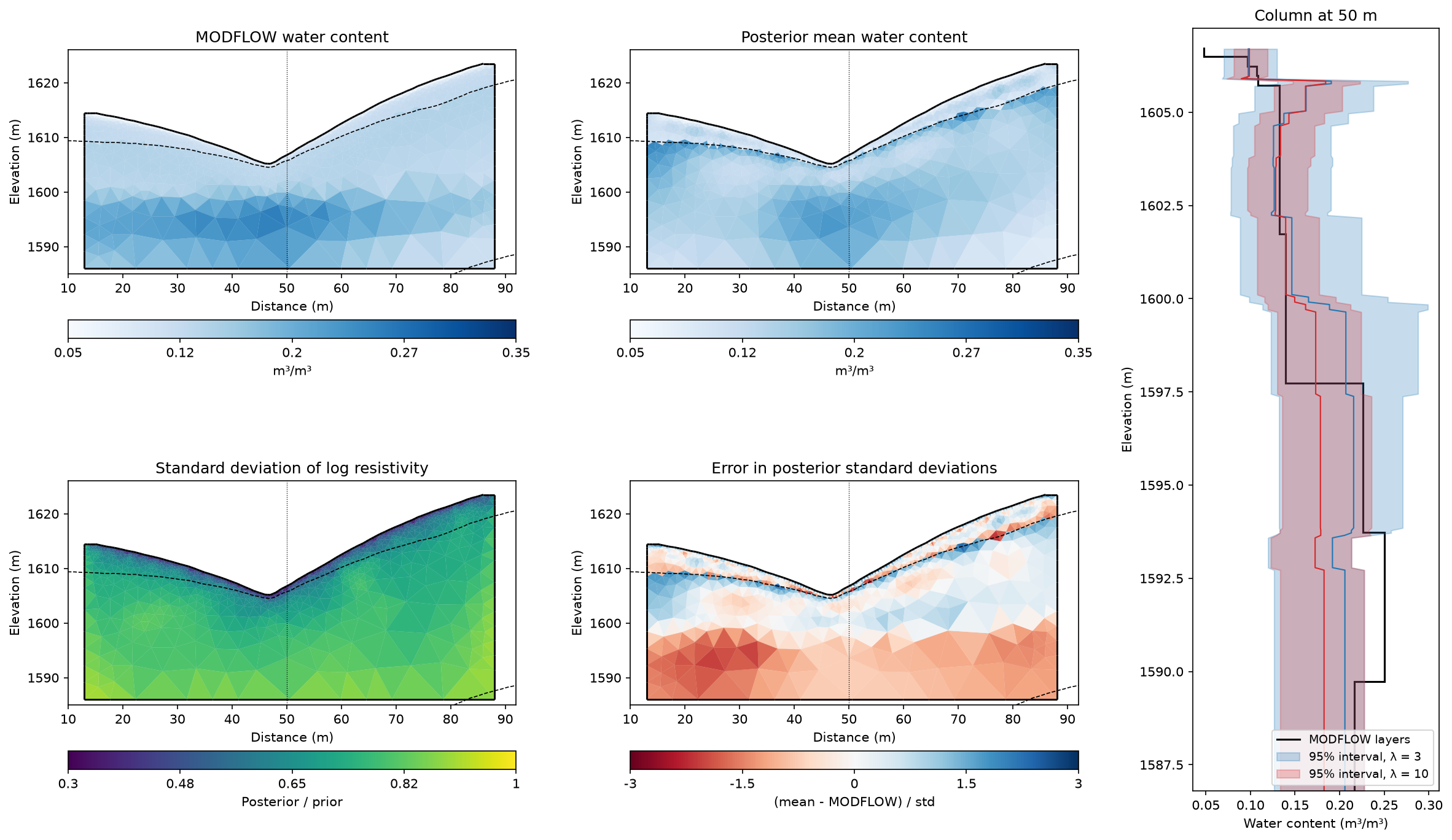
The maps are for lambda=3. The column on the right follows the dotted line at 50 m: the MODFLOW layers, and the 95% intervals at both prior strengths.

output_dir = os.path.join(current_dir, "results", "posterior_uncertainty")
os.makedirs(output_dir, exist_ok=True)
chosen = posteriors[3.]
np.savez_compressed(os.path.join(output_dir, "posterior.npz"),
                    cell_centers=np.array(cells.cellCenters()), unit=unit,
                    modflow_water_content=modflow_theta, posterior_cov=chosen["posterior_cov"],
                    **{f"{key}_lambda{lam:g}": value for lam, posterior in posteriors.items()
                       for key, value in posterior.items() if key not in ("cells", "posterior_cov")})
chosen_std = np.sqrt(np.diag(chosen["posterior_cov"]))
fig = plt.figure(figsize=(16, 9))
grid = fig.add_gridspec(2, 3, width_ratios=[1, 1, .55], left=.05, right=.98, top=.96,
                        bottom=.04, wspace=.3, hspace=.3)
maps = [
    (grid[0, 0], modflow_theta, dict(cMap="Blues", cMin=.05, cMax=.35, label="m³/m³"),
     "MODFLOW water content"),
    (grid[0, 1], chosen["mean"], dict(cMap="Blues", cMin=.05, cMax=.35, label="m³/m³"),
     "Posterior mean water content"),
    (grid[1, 0], chosen_std / chosen["prior_std"], dict(cMap="viridis", cMin=.3, cMax=1.,
                                                       label="Posterior / prior"),
     "Standard deviation of log resistivity"),
    (grid[1, 1], (chosen["mean"] - modflow_theta) / chosen["std"],
     dict(cMap="RdBu", cMin=-3, cMax=3, label="(mean - MODFLOW) / std"),
     "Error in posterior standard deviations"),
]
for position, values, style, title in maps:
    ax = fig.add_subplot(position)
    pg.show(cells, values, ax=ax, orientation="horizontal", **style)
    for line in (regolith_base, fractured_base):
        ax.plot(*line.T, "k--", lw=.8)
    ax.axvline(50., color="k", lw=.6, ls=":")
    ax.set(title=title, xlim=(10, 92), ylim=(1585, 1626), xlabel="Distance (m)",
           ylabel="Elevation (m)")
column = np.argmin(np.abs(interpolator.L_profile - 50.))
elevation = np.linspace(structure[0, column] - .05, z.min(), 300)
hits = [cells.findCell(pg.Pos(50., e)) for e in elevation]
keep = np.array([cell is not None for cell in hits])
ids = np.array([cell.id() for cell in hits if cell is not None])
ax = fig.add_subplot(grid[:, 2])
ax.stairs(profile_water_content[::-1, column], structure[::-1, column], orientation="horizontal",
          baseline=None, color="k", lw=1.5, label="MODFLOW layers")
for lam, color in [(3., "C0"), (10., "C3")]:
    posterior = posteriors[lam]
    ax.fill_betweenx(elevation[keep], posterior["low"][ids], posterior["high"][ids], color=color,
                     alpha=.25, label=f"95% interval, λ = {lam:g}")
    ax.plot(posterior["mean"][ids], elevation[keep], color=color, lw=1)
ax.set(ylim=(z.min(), structure[0, column] + .5), xlabel="Water content (m³/m³)",
       ylabel="Elevation (m)", title="Column at 50 m")
ax.legend(loc="lower right", fontsize=9)
fig.savefig(os.path.join(output_dir, "posterior_uncertainty.png"), dpi=150, bbox_inches="tight")
plt.show()

The survey reduces the standard deviation of log resistivity most near the surface (bottom left): to a median of 0.55 of its prior value in the regolith, against 0.74 in the fractured bedrock. Through the fixed petrophysics, the lambda=3 posterior gives 95% intervals about 0.09 m³/m³ wide in the regolith and 0.14 in the fractured bedrock, and they contain the MODFLOW water content in 99% of both units. The errors are not random, though (bottom centre): the smooth section underestimates the water content of the saturated bedrock below the water table and errs both ways along the base of the regolith, where it blurs the MODFLOW interfaces. The stronger prior (lambda=10) fits the survey a little worse (chi-squared 1.09 against 0.93) and returns intervals about 40% narrower, which contain the MODFLOW state in only 80-84% of the section (right). Linearized intervals are only as reliable as the regularization they inherit, so choose lambda by the data misfit, and read the intervals as conditional on the petrophysics and the unit boundaries.