Synthetic LM+HM line inversion with lateral constraints.

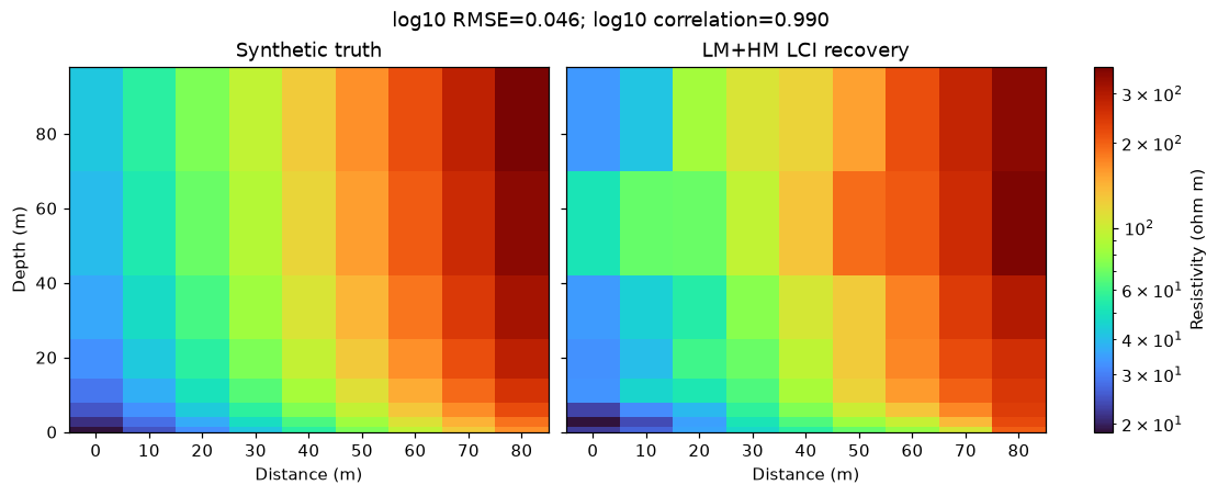
This example loads the bundled nine-station SQLite project through the same TEMcompany/TEM2Go reader used by the Qt Studio. It jointly fits the LM and HM gates, applies same-line L2 lateral constraints, and compares the recovered section with the known synthetic resistivity model.

Because the truth model is known, the run doubles as an accuracy check: it reports a log10 RMSE and a correlation against the truth, so a regression in the 1D forward model or in the lateral constraint shows up as a number rather than as a section that merely looks plausible.

from __future__ import annotations

import numpy as np
import matplotlib.pyplot as plt
from matplotlib.colors import LogNorm

from PyHydroGeophysX.workflows import em1d


def run_example() -> tuple[dict, float, float]:
    """Run the bundled line inversion and return result, RMSE, and correlation."""
    spec = em1d.example_catalog()["synthetic_tem_lci"]
    project = spec["path"]
    truth = np.load(project / "truth_model.npy")
    head = em1d.load_sounding(str(project), "TDEM", moment="LM+HM")

    geometry = {**head["system"], "tem_moment": "LM+HM"}
    inversion = {
        **em1d.DEFAULT_INVERSION,
        **head["inversion_defaults"],
        **spec["params"],
    }
    result = em1d.invert_line(
        str(project),
        "TDEM",
        geometry,
        inversion,
        positions=np.asarray(head["positions"], dtype=float),
        heights=np.asarray(head["heights"], dtype=float),
        max_soundings=truth.shape[0],
        doi_blank=False,
    )
    recovered = np.asarray(result["model3d"][:, 0, ::-1], dtype=float)
    log_truth = np.log10(truth)
    log_recovered = np.log10(recovered)
    log_rmse = float(np.sqrt(np.mean((log_recovered - log_truth) ** 2)))
    correlation = float(np.corrcoef(
        log_truth.ravel(), log_recovered.ravel())[0, 1])
    return result, log_rmse, correlation


def plot_result(result: dict, log_rmse: float, correlation: float) -> None:
    """Plot the true and recovered resistivity sections on a shared scale."""
    spec = em1d.example_catalog()["synthetic_tem_lci"]
    truth = np.load(spec["path"] / "truth_model.npy")
    recovered = np.asarray(result["model3d"][:, 0, ::-1], dtype=float)
    thickness = np.asarray(result["thickness"], dtype=float)
    depth_edges = np.concatenate([
        [0.0], np.cumsum(thickness),
        [float(np.sum(thickness) + thickness[-1])],
    ])
    positions = np.asarray(result["positions"], dtype=float)
    position_edges = np.concatenate([
        [positions[0] - 5.0],
        0.5 * (positions[:-1] + positions[1:]),
        [positions[-1] + 5.0],
    ])
    norm = LogNorm(vmin=float(np.min(truth)), vmax=float(np.max(truth)))

    # Constrained layout, because a colorbar spanning both axes is one of the
    # cases tight_layout cannot solve: it warns and then draws the bar on top of
    # the right-hand panel.
    fig, axes = plt.subplots(
        1, 2, figsize=(10, 4), sharey=True, layout="constrained")
    for axis, values, title in zip(
        axes, (truth, recovered), ("Synthetic truth", "LM+HM LCI recovery")
    ):
        image = axis.pcolormesh(
            position_edges, depth_edges, values.T,
            shading="flat", cmap="turbo", norm=norm)
        axis.invert_yaxis()
        axis.set_title(title)
        axis.set_xlabel("Distance (m)")
    axes[0].set_ylabel("Depth (m)")
    fig.colorbar(image, ax=axes, label="Resistivity (ohm m)")
    fig.suptitle(
        f"log10 RMSE={log_rmse:.3f}; log10 correlation={correlation:.3f}")
    plt.show()


if __name__ == "__main__":
    inversion_result, model_rmse, model_correlation = run_example()
    print(f"Mean data chi2: {inversion_result['chi2']:.3f}")
    print(f"Model log10 RMSE: {model_rmse:.3f}")
    print(f"Model log10 correlation: {model_correlation:.3f}")
    plot_result(inversion_result, model_rmse, model_correlation)

Recovered Section Against the Truth

The two panels share a logarithmic colour scale, so a colour that matches between them is a resistivity that matches. The nine-station line recovers the lateral gradient and the shallow conductive layer; depth resolution softens below roughly 60 m, which is where the late gates stop constraining the model.

The bundled run reports a mean data chi-square near 0.86, a log10 RMSE of 0.046 against the truth model, and a correlation of 0.990.