Ex. Airborne EM Line Inversion#

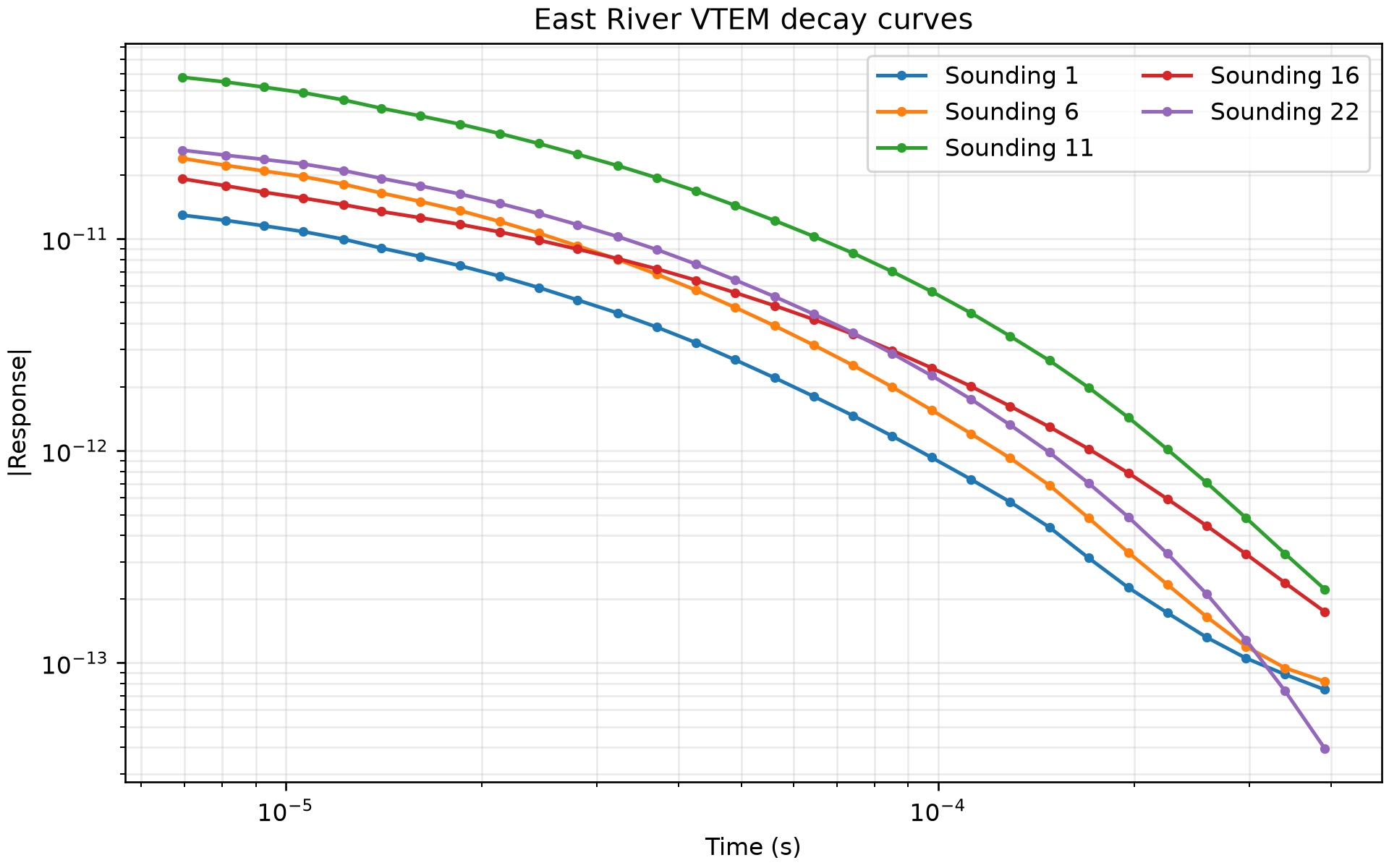
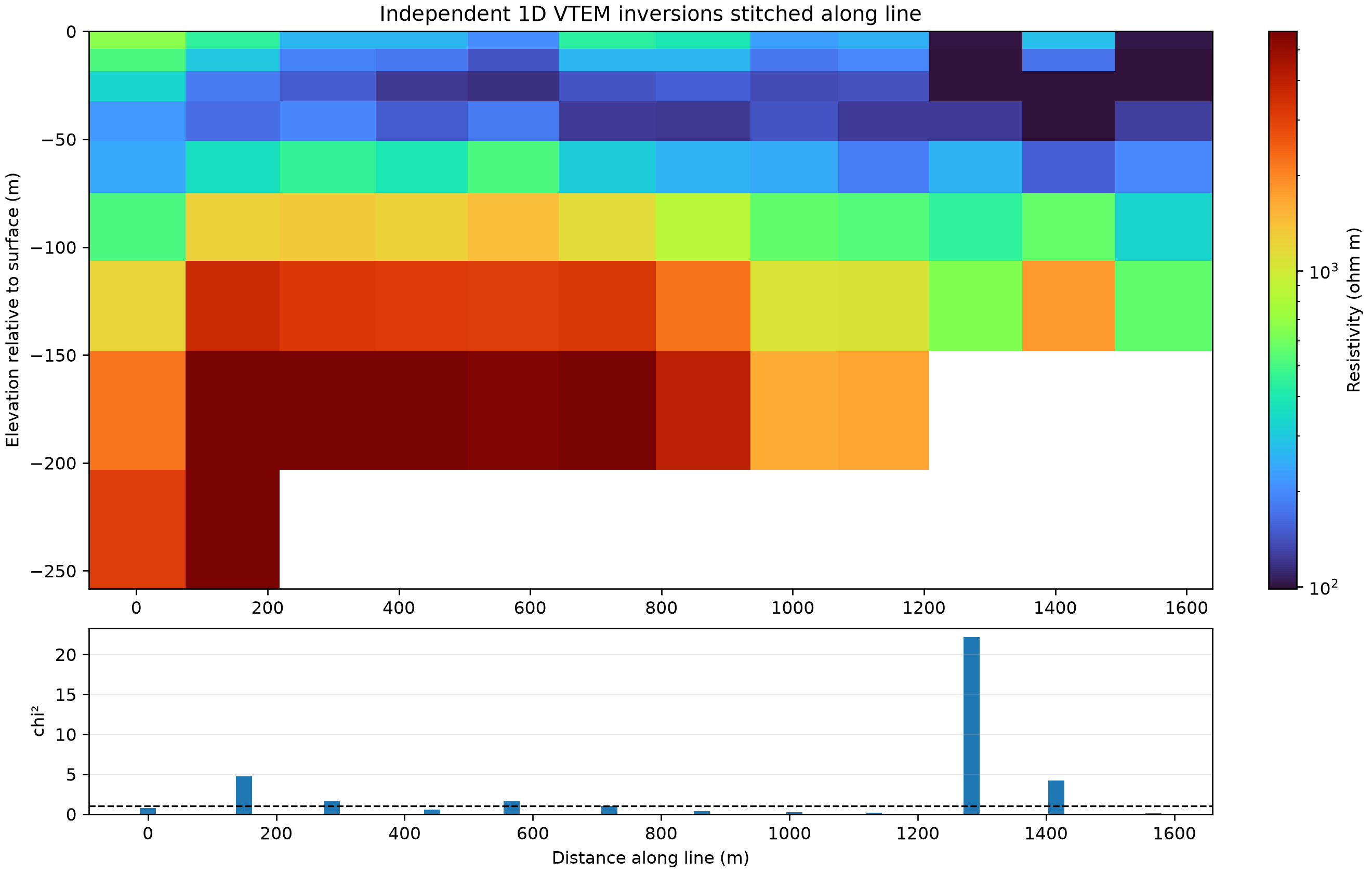
This example loads a VTEM line and its survey geometry, inspects measured decays, calibrates the response to a documented reference resistivity, and creates a stitched resistivity section from independent 1D inversions.

from pathlib import Path
import sys

current_dir = Path(__file__).resolve().parent if "__file__" in globals() else Path.cwd()
repo_root = current_dir.parent
if str(repo_root) not in sys.path:
    sys.path.insert(0, str(repo_root))

import matplotlib.pyplot as plt
from matplotlib.colors import LogNorm
import numpy as np
import pandas as pd

from PyHydroGeophysX.workflows.em1d import (
    calibrate_to_reference,
    invert_line,
    load_line_geometry,
    load_sounding,
)


data_dir = current_dir / "data" / "EM" / "EastRiver_VTEM"
output_dir = current_dir / "results" / "em_line_section"
output_dir.mkdir(parents=True, exist_ok=True)
data_path = data_dir / "eastriver_vtem_line22030.csv"
geometry_path = data_dir / "eastriver_vtem_line22030_geometry.csv"

Inspect the VTEM Soundings#

geometry = load_line_geometry(str(geometry_path))
fig, ax = plt.subplots(figsize=(8, 5), constrained_layout=True)
for sounding in (0, 5, 10, 15, 21):
    data = load_sounding(str(data_path), "TDEM", sounding=sounding)
    ax.loglog(data["times"], np.abs(data["response"]), marker="o", ms=3,
              label=f"Sounding {sounding + 1}")
ax.set_xlabel("Time (s)")
ax.set_ylabel("|Response|")
ax.set_title("East River VTEM decay curves")
ax.grid(True, which="both", alpha=0.25)
ax.legend(ncols=2)
fig.savefig(output_dir / "Ex_EM_line_section_fig_01.png", dpi=240)
plt.show()

print(f"Loaded {load_sounding(str(data_path), 'TDEM')['n_soundings']} soundings")
print(f"Line distance: {geometry['positions'].min():.1f}–{geometry['positions'].max():.1f} m")

../_images/Ex_EM_line_section_fig_01.png

Calibrate and Invert the Line#

The documented 320 ohm-m reference constrains the otherwise ambiguous amplitude scale. Twelve soundings are used here to keep the tutorial compact.

forward_geometry = {
    "source_radius": 13.0,
    "height": 82.0,
    "orientation": "z",
    "waveform": "step_off",
}
inversion_parameters = {
    "n_layers": 9,
    "min_thickness": 8.0,
    "max_thickness": 55.0,
    "starting_resistivity": 320.0,
    "smoothness": 0.5,
    "rel_error": 0.08,
    "max_iterations": 6,
}
data_scale = calibrate_to_reference(
    str(data_path), "TDEM", forward_geometry, inversion_parameters,
    ref_resistivity=320.0, max_probe=4,
)
inversion_parameters["data_scale"] = data_scale
result = invert_line(
    str(data_path), "TDEM", forward_geometry, inversion_parameters,
    positions=geometry["positions"], heights=geometry["heights"],
    max_soundings=12, doi_blank=True, out_dir=output_dir,
)

ex, _, ez = result["edges"]
section = np.asarray(result["model3d"])[:, 0, :].T
finite = section[np.isfinite(section) & (section > 0)]
vmin, vmax = np.nanpercentile(finite, [5, 95])

fig, axes = plt.subplots(2, 1, figsize=(11, 7), constrained_layout=True,
                         gridspec_kw={"height_ratios": [3, 1]})
image = axes[0].pcolormesh(ex, ez, section, shading="auto", cmap="turbo",
                           norm=LogNorm(vmin=max(vmin, 1.0), vmax=vmax))
fig.colorbar(image, ax=axes[0], label="Resistivity (ohm m)")
axes[0].set_ylabel("Elevation relative to surface (m)")
axes[0].set_title("Independent 1D VTEM inversions stitched along line")
chi2 = np.asarray(result["chi2_list"], dtype=float)
axes[1].bar(result["positions"], chi2, width=25.0, color="tab:blue")
axes[1].axhline(1.0, color="k", ls="--", lw=1)
axes[1].set_xlabel("Distance along line (m)")
axes[1].set_ylabel("chi²")
axes[1].grid(axis="y", alpha=0.25)
fig.savefig(output_dir / "Ex_EM_line_section_fig_02.png", dpi=240)
plt.show()

print(f"Calibration scale: {data_scale:.4g}")
print(f"Mean line chi2: {result['chi2']:.3f}")

../_images/Ex_EM_line_section_fig_02.png

Compare with the Published Reference Section#

The comparison is restricted to the shallowest 100 m, which is what this data set can support. The recorded gates stop at 391 microseconds, giving a diffusion depth near 450 m in a 320 ohm-m half-space, and sensitivity has already fallen off well above that. The published USGS section extends to 1000 m; below roughly 100 m the inversion here drifts progressively resistive (a factor of four by 200 m) because the late-time data that would hold it down were never recorded. Comparing the full depth range would say more about that missing sensitivity than about either inversion.

The amplitude is a second reason to read this as a check rather than a validation: calibrate_to_reference sets the data scale by assuming a 320 ohm-m half-space, so it is an assumption, not an instrument calibration.

COMPARISON_DEPTH_M = 100.0

reference = pd.read_csv(data_dir / "eastriver_vtem_line22030_usgs_resistivity.csv")
reference_depth = reference.iloc[:, 0].to_numpy(float)
reference_model = reference.iloc[:, 1:13].to_numpy(float)
positions = np.asarray(result["positions"], dtype=float)
depth_center = -0.5 * (ez[:-1] + ez[1:])

# Both grids ordered by increasing depth, then cut at the comparison depth.
order = np.argsort(depth_center)
depth_center, section_sorted = depth_center[order], section[order]
ours_band = depth_center <= COMPARISON_DEPTH_M
ref_band = reference_depth <= COMPARISON_DEPTH_M

# One colour scale for both panels, taken from both panels. Scaling it to this
# inversion alone (as a percentile of `section`) pushes the reference into the
# bottom of the colour map and hides its structure.
paired = np.concatenate([
    section_sorted[ours_band].ravel(), reference_model[ref_band].ravel()])
paired = paired[np.isfinite(paired) & (paired > 0)]
norm = LogNorm(*np.nanpercentile(paired, [2, 98]))

fig, axes = plt.subplots(1, 2, figsize=(12, 5), constrained_layout=True, sharey=True)
axes[0].pcolormesh(positions, depth_center[ours_band],
                   section_sorted[ours_band], shading="nearest",
                   cmap="turbo", norm=norm)
axes[0].set_title("PyHydroGeophysX")
axes[0].set_xlabel("Distance (m)")
axes[0].set_ylabel("Depth (m)")
ref_image = axes[1].pcolormesh(positions, reference_depth[ref_band],
                               reference_model[ref_band], shading="nearest",
                               cmap="turbo", norm=norm)
axes[1].set_title("Provided USGS reference")
axes[1].set_xlabel("Distance (m)")
axes[0].set_ylim(COMPARISON_DEPTH_M, 0)
fig.colorbar(ref_image, ax=axes, label="Resistivity (ohm m)")
fig.suptitle(f"Upper {COMPARISON_DEPTH_M:.0f} m, the depth range these gates constrain")
fig.savefig(output_dir / "Ex_EM_line_section_fig_03.png", dpi=240)
plt.show()

# Score the overlap instead of leaving the reader to judge two colour maps.
on_reference = np.full((ref_band.sum(), section_sorted.shape[1]), np.nan)
for column in range(section_sorted.shape[1]):
    trace = section_sorted[:, column]
    usable = np.isfinite(trace) & (trace > 0)
    if usable.sum() >= 2:
        on_reference[:, column] = np.interp(
            reference_depth[ref_band], depth_center[usable], trace[usable],
            left=np.nan, right=np.nan)
comparable = np.isfinite(on_reference) & np.isfinite(reference_model[ref_band])
ours_log = np.log10(on_reference[comparable])
theirs_log = np.log10(reference_model[ref_band][comparable])
print(f"Upper {COMPARISON_DEPTH_M:.0f} m, {comparable.sum()} comparable cells")
print(f"  log10 RMSE vs USGS: {np.sqrt(np.mean((ours_log - theirs_log) ** 2)):.3f}"
      f"  (0.30 is a factor of two)")
print(f"  median resistivity: {10 ** np.median(ours_log):.0f} ohm m here, "
      f"{10 ** np.median(theirs_log):.0f} ohm m in the reference")

# Per band, so the depth at which agreement decays is visible as a number.
print("  by depth band:")
for lower, upper in ((0.0, 40.0), (40.0, 70.0), (70.0, COMPARISON_DEPTH_M)):
    rows = (reference_depth[ref_band] >= lower) & (reference_depth[ref_band] < upper)
    cells = comparable[rows]
    if cells.sum() < 3:
        continue
    band_ours = np.log10(on_reference[rows][cells])
    band_theirs = np.log10(reference_model[ref_band][rows][cells])
    print(f"    {lower:>3.0f}-{upper:>3.0f} m: "
          f"log10 RMSE {np.sqrt(np.mean((band_ours - band_theirs) ** 2)):.3f}, "
          f"median {10 ** np.median(band_ours):>4.0f} vs "
          f"{10 ** np.median(band_theirs):.0f} ohm m")

../_images/Ex_EM_line_section_fig_03.png

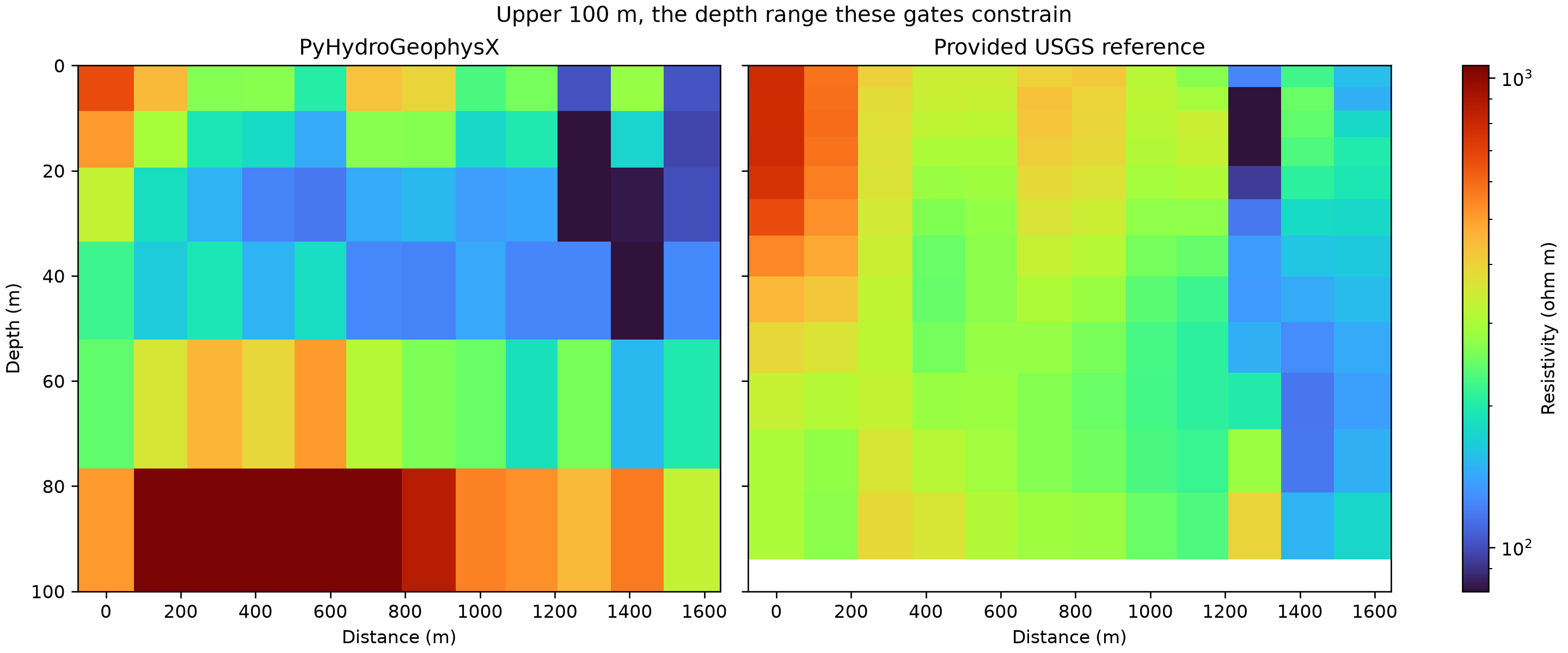
Agreement is closest between about 40 and 70 m, where the two sections differ by a factor of 1.5 (log10 RMSE 0.167, medians 211 and 257 ohm-m). Over the whole upper 100 m it is a factor of two (log10 RMSE 0.274), which is what to expect from independent 1D inversions using different codes, layer grids and regularization. Both sections also place the same near-surface conductor around 1200 to 1400 m along the line.

The deepest row drawn here is the layer centred at 91 m, and it is already running high: 523 ohm-m against 280 in the reference. That row is the start of the resistive drift described above, so read the bottom of this figure as the edge of the usable range rather than as a result.