Note
Go to the end to download the full example code.
Ex. Time-Lapse ERT Inversion Techniques#
This example demonstrates different approaches for time-lapse electrical resistivity tomography (ERT) inversion using PyHydroGeophysX.
The example includes: 1. Full time-lapse inversion with temporal regularization 2. Windowed time-lapse inversion for large datasets 3. L1-norm regularized inversion for sharp boundary recovery 4. Comparison of different inversion strategies 5. Visualization of resistivity evolution over time
Time-lapse ERT inversion is crucial for monitoring subsurface water content changes and understanding hydrological processes in watersheds. The temporal regularization helps maintain consistency between consecutive time steps while allowing for realistic changes.
import os
import sys
import numpy as np
import matplotlib.pyplot as plt
import pygimli as pg
from pygimli.physics import ert
from mpl_toolkits.axes_grid1 import make_axes_locatable

# Setup package path for development
try:
    # For regular Python scripts
    current_dir = os.path.dirname(os.path.abspath(__file__))
except NameError:
    # For Jupyter notebooks
    current_dir = os.getcwd()

# Add the parent directory to Python path
parent_dir = os.path.dirname(current_dir)
if parent_dir not in sys.path:
    sys.path.append(parent_dir)

# Import PyHydroGeophysX modules
from PyHydroGeophysX.inversion.time_lapse import TimeLapseERTInversion
from PyHydroGeophysX.inversion.windowed import WindowedTimeLapseERTInversion
data_dir = os.path.join(current_dir, "data", "TL_measurements", "appres")

# List of ERT data files testing monthly time-lapse inversion
ert_files = [
    "synthetic_data30.dat",
    "synthetic_data60.dat",
    "synthetic_data90.dat",
    "synthetic_data120.dat",
    "synthetic_data150.dat",
    "synthetic_data180.dat",
    "synthetic_data210.dat",
    "synthetic_data240.dat",
    "synthetic_data270.dat",
    "synthetic_data300.dat",
    "synthetic_data330.dat",
    "synthetic_data360.dat",
]
## 1.Full L2 Time-Lapse Inversion
#################### FUll Time-Lapse Inversion #####################
# Full paths to data files
data_files = [os.path.join(data_dir, f) for f in ert_files]

# Measurement times (can be timestamps or any sequential numbers representing time)
measurement_times = [1, 2, 3, 4, 5, 6, 7 ,8, 9, 10, 11, 12]  # Adjust based on your actual acquisition times

# Create a mesh for the inversion (or load an existing one)
data = ert.load(data_files[0])
ert_manager = ert.ERTManager(data)
mesh = ert_manager.createMesh(data=data, quality=34)

# Set up inversion parameters
inversion_params = {
    "lambda_val": 50.0,              # Regularization parameter
    "alpha": 10.0,                   # Temporal regularization parameter
    "decay_rate": 0.0,               # Temporal decay rate
    "method": "cgls",                # Solver method ('cgls', 'lsqr', etc.)
    "model_constraints": (0.001, 1e4), # Min/max resistivity values (ohm-m)
    "max_iterations": 15,            # Maximum iterations
    "absoluteUError": 0.0,           # Absolute data error (V)
    "relativeError": 0.05,           # Relative data error (5%)
    "lambda_rate": 1.0,              # Lambda reduction rate
    "lambda_min": 1.0,               # Minimum lambda value
    "inversion_type": "L2"           # 'L1', 'L2', or 'L1L2'
}

# Create the time-lapse inversion object
inversion = TimeLapseERTInversion(
    data_files=data_files,
    measurement_times=measurement_times,
    mesh=mesh,
    **inversion_params
)

# Run the inversion
print("Starting time-lapse inversion...")
result = inversion.run()
print("Inversion complete!")
from palettable.lightbartlein.diverging import BlueDarkRed18_18
fixed_cmap = BlueDarkRed18_18.mpl_colormap

fig = plt.figure(figsize=[16,6])

# True resistivity model
for i in range(12):
    ax = fig.add_subplot(3,4,i+1)
    ax, cbar = pg.show(result.mesh,result.final_models[:,i],pad=0.3,orientation="vertical",cMap=fixed_cmap,cMin= 100,cMax = 3000
                    , ylabel="Elevation (m)",label=r' Resistivity ($\Omega$ m)',ax=ax,logScale=False,coverage=result.all_coverage[i]>-1)
    cbar.remove()
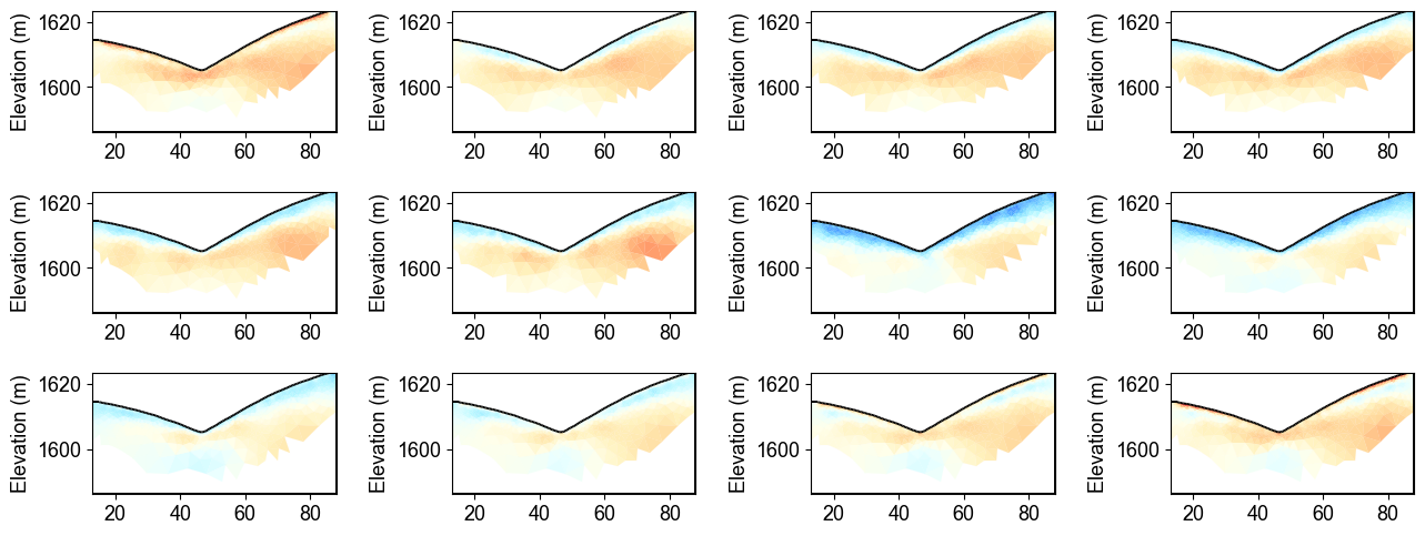
Full Time-Lapse ERT Inversion Results#
The time-lapse sequence reveals the temporal evolution of subsurface water content over 12 months. Notice how the resistivity distribution changes systematically, with high resistivity zones (dry areas) gradually becoming more conductive (wet) as water infiltrates through the soil layers. The temporal regularization ensures smooth transitions between consecutive time steps while capturing realistic subsurface changes.
## 2. Window L2 time-lapse inversion
Measurement times (can be timestamps or any sequential numbers representing time)
measurement_times = [1, 2, 3, 4, 5, 6, 7, 8, 9, 10, 11, 12]  # Adjust based on your actual acquisition times

# Create a mesh for the inversion (or load an existing one)
data = ert.load(os.path.join(data_dir, ert_files[0]))
ert_manager = ert.ERTManager(data)
mesh = ert_manager.createMesh(data=data, quality=34)

# Set up inversion parameters
inversion_params = {
    "lambda_val": 10.0,              # Regularization parameter
    "alpha": 10.0,                   # Temporal regularization parameter
    "decay_rate": 0.0,               # Temporal decay rate
    "method": "cgls",                # Solver method ('cgls', 'lsqr', etc.)
    "model_constraints": (0.001, 1e4), # Min/max resistivity values (ohm-m)
    "max_iterations": 15,            # Maximum iterations
    "absoluteUError": 0.0,           # Absolute data error (V)
    "relativeError": 0.05,           # Relative data error (5%)
    "lambda_rate": 1.0,              # Lambda reduction rate
    "lambda_min": 1.0,               # Minimum lambda value
    "inversion_type": "L2"           # 'L1', 'L2', or 'L1L2'
}

# Define the window size (number of timesteps to process together)
window_size = 3  # A window size of 3 means each window includes 3 consecutive measurements

# Create the windowed time-lapse inversion object
inversion = WindowedTimeLapseERTInversion(
    data_dir=data_dir,               # Directory containing ERT data files
    ert_files=ert_files,             # List of ERT data filenames
    measurement_times=measurement_times,  # List of measurement times
    window_size=window_size,         # Size of sliding window
    mesh=mesh,                       # Mesh for inversion
    **inversion_params               # Pass the same inversion parameters
)

# Run the inversion, optionally in parallel
print("Starting windowed time-lapse inversion...")
result = inversion.run()
print("Inversion complete!")
result.final_models = np.array(result.final_models)
result.final_models.shape
from palettable.lightbartlein.diverging import BlueDarkRed18_18
import matplotlib.pyplot as plt
import numpy as np
import matplotlib.pylab as pylab
params = {'legend.fontsize': 13,
          #'figure.figsize': (15, 5),
         'axes.labelsize': 13,
         'axes.titlesize':13,
         'xtick.labelsize':13,
         'ytick.labelsize':13}

pylab.rcParams.update(params)
plt.rcParams["font.family"] = "Arial"

fixed_cmap = BlueDarkRed18_18.mpl_colormap
fig = plt.figure(figsize=[16, 6])

# Use tight_layout with adjusted parameters to reduce space
plt.subplots_adjust(wspace=0.05, hspace=0.05)

# True resistivity model
for i in range(12):
    row, col = i // 4, i % 4
    ax = fig.add_subplot(3, 4, i+1)

    # Add common ylabel only to leftmost panels
    ylabel = "Elevation (m)" if col == 0 else None

    # Add resistivity label only to the middle-right panel (row 1, col 3)
    resistivity_label = r' Resistivity ($\Omega$ m)' if (i == 7) else None

    # Only show axis ticks on leftmost and bottom panels
    if col != 0:
        ax.set_yticks([])

    if row != 2:  # Not bottom row
        ax.set_xticks([])
    else:
        # Add "distance (m)" label to bottom row panels
        ax.set_xlabel("Distance (m)")

    # Create the plot
    ax, cbar = pg.show(result.mesh,
                      result.final_models[:,i],
                      pad=0.3,
                      orientation="vertical",
                      cMap=fixed_cmap,
                      cMin=100,
                      cMax=3000,
                      ylabel=ylabel,
                      label=resistivity_label,
                      ax=ax,
                      logScale=False,
                      coverage=result.all_coverage[i]>-1.2)

    # Only keep colorbar for the middle-right panel (row 1, col 3)
    # This corresponds to panel index 7 in a 0-based indexing system
    if i != 7:  # Keep only the colorbar for panel 7
        cbar.remove()

plt.tight_layout()
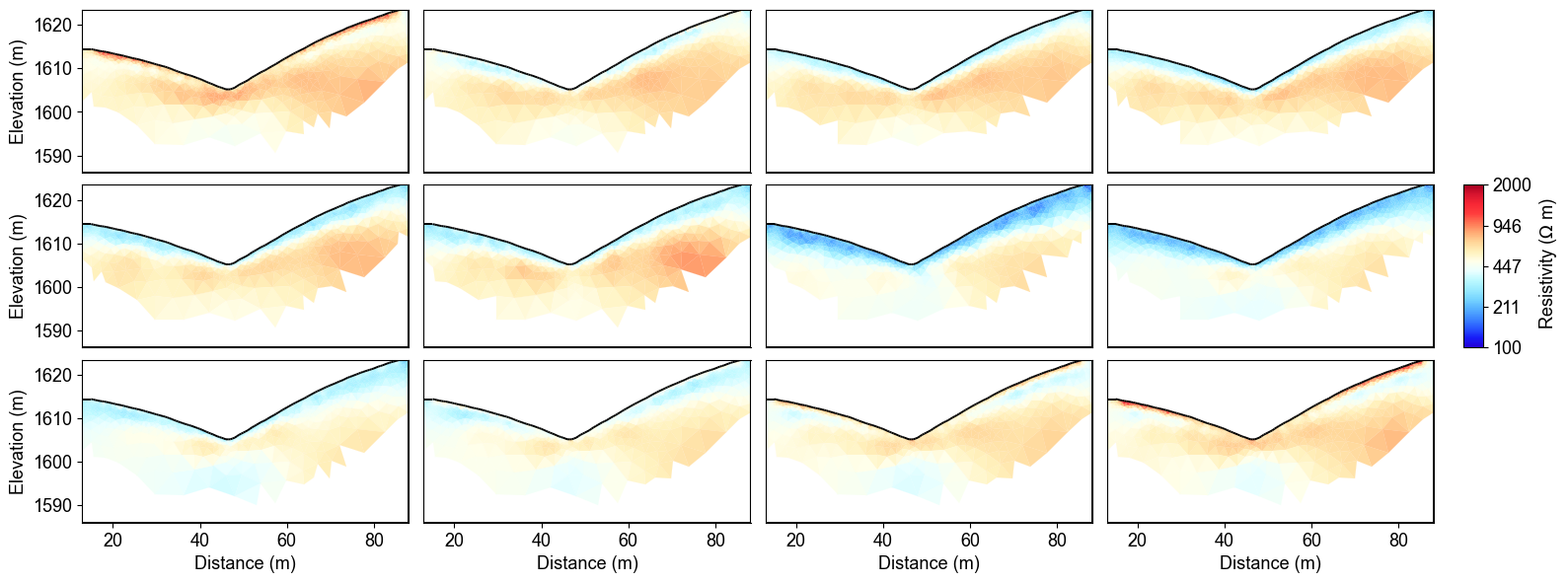
Windowed Time-Lapse Inversion Results#
The windowed approach processes consecutive time steps in overlapping groups, which is computationally more efficient for large datasets while maintaining temporal coherence. This method shows similar overall patterns to the full time-lapse inversion but with reduced computational cost. The windowing approach is particularly valuable when processing years of monitoring data or when computational resources are limited.
## 3. Full L1 Time-lapse Inversion
ax, cbar = pg.show(result.mesh,result.final_models[:,i],pad=0.3,orientation="vertical",cMap=fixed_cmap,cMin= 100,cMax = 3000
                    , ylabel="Elevation (m)",label=r' Resistivity ($\Omega$ m)',logScale=False,coverage=result.all_coverage[i]>-1)
Full paths to data files
data_files = [os.path.join(data_dir, f) for f in ert_files]

# Measurement times (can be timestamps or any sequential numbers representing time)
measurement_times = [1, 2, 3, 4, 5, 6, 7 ,8, 9, 10, 11, 12]  # Adjust based on your actual acquisition times

# Create a mesh for the inversion (or load an existing one)
data = ert.load(data_files[0])
ert_manager = ert.ERTManager(data)
mesh = ert_manager.createMesh(data=data, quality=34)

# Set up inversion parameters
inversion_params = {
    "lambda_val": 50.0,              # Regularization parameter
    "alpha": 10.0,                   # Temporal regularization parameter
    "decay_rate": 0.0,               # Temporal decay rate
    "method": "cgls",                # Solver method ('cgls', 'lsqr', etc.)
    "model_constraints": (0.001, 1e4), # Min/max resistivity values (ohm-m)
    "max_iterations": 15,            # Maximum iterations
    "absoluteUError": 0.0,           # Absolute data error (V)
    "relativeError": 0.05,           # Relative data error (5%)
    "lambda_rate": 1.0,              # Lambda reduction rate
    "lambda_min": 1.0,               # Minimum lambda value
    "inversion_type": "L1"           # 'L1', 'L2', or 'L1L2'
}

# Create the time-lapse inversion object
inversion = TimeLapseERTInversion(
    data_files=data_files,
    measurement_times=measurement_times,
    mesh=mesh,
    **inversion_params
)

# Run the inversion
print("Starting time-lapse inversion...")
result_L1 = inversion.run()
print("Inversion complete!")
from palettable.lightbartlein.diverging import BlueDarkRed18_18
fixed_cmap = BlueDarkRed18_18.mpl_colormap

fig = plt.figure(figsize=[16,6])

# True resistivity model
for i in range(12):
    ax = fig.add_subplot(3,4,i+1)
    ax, cbar = pg.show(result_L1.mesh,result_L1.final_models[:,i],pad=0.3,orientation="vertical",cMap=fixed_cmap,cMin= 100,cMax = 3000
                    , ylabel="Elevation (m)",label=r' Resistivity ($\Omega$ m)',ax=ax,logScale=False,coverage=result.all_coverage[i]>-1)
    cbar.remove()
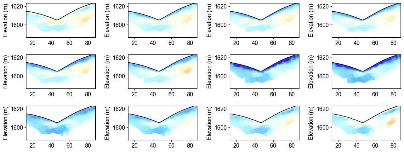
L1-Norm Regularized Inversion Results#
The L1-norm regularization produces sharper boundaries compared to L2 regularization, which is beneficial for detecting distinct geological layers or sharp interfaces. Notice how the resistivity transitions are more abrupt in this inversion, making it easier to identify distinct zones of different water content. This approach is particularly useful when the subsurface is expected to have layered structures rather than gradual transitions.
Summary and Recommendations#
This example demonstrated three approaches to time-lapse ERT inversion:
Key Findings:
Temporal regularization is essential for realistic time-lapse results
Windowed inversion provides computational efficiency with minimal quality loss
L1 regularization enhances boundary detection in layered media
Parameter tuning (λ, α) significantly affects result quality
Recommendations:
Use full L2 for high-quality results with moderate datasets
Apply windowed L2 for large datasets or real-time processing
Choose L1 regularization when sharp interfaces are expected
Always validate results against known geological information
Next Steps:
Combine with seismic constraints (see structure-constrained examples)
Apply uncertainty quantification (see Monte Carlo examples)
Integrate with hydrological models for enhanced interpretation