Ex. Creating Synthetic Time-Lapse ERT Measurements

This example demonstrates how to create synthetic time-lapse electrical resistivity tomography (ERT) measurements for watershed monitoring applications.

The example covers: 1. Loading time-series water content data from MODFLOW simulations 2. Converting water content to resistivity for each timestep 3. Forward modeling to generate synthetic ERT data for multiple time periods 4. Parallel processing for efficient computation across multiple timesteps 5. Visualization of apparent resistivity changes over time 6. Creating animations showing temporal water content variations

This workflow is essential for testing time-lapse inversion algorithms and understanding the sensitivity of ERT measurements to hydrological changes.

import os
import sys
import numpy as np
import matplotlib.pyplot as plt
import pygimli as pg
from pygimli.physics import ert
from mpl_toolkits.axes_grid1 import make_axes_locatable

# Setup package path for development
try:
    # For regular Python scripts
    current_dir = os.path.dirname(os.path.abspath(__file__))
except NameError:
    # For Jupyter notebooks
    current_dir = os.getcwd()

# Add the parent directory to Python path
parent_dir = os.path.dirname(current_dir)
if parent_dir not in sys.path:
    sys.path.append(parent_dir)

# Import PyHydroGeophysX modules
from PyHydroGeophysX.model_output.modflow_output import MODFLOWWaterContent
from PyHydroGeophysX.core.interpolation import ProfileInterpolator, create_surface_lines
from PyHydroGeophysX.core.mesh_utils import MeshCreator
from PyHydroGeophysX.petrophysics.resistivity_models import water_content_to_resistivity
from PyHydroGeophysX.forward.ert_forward import ERTForwardModeling

output_dir = os.path.join(current_dir,  "results", "TL_measurements") #"C:/Users/HChen8/Documents/GitHub/PyHydroGeophysX/examples/results/TL_measurements"
os.makedirs(output_dir, exist_ok=True)

print("Step 1: Set up the ERT profiles like in the workflow example.")

data_dir = os.path.join(current_dir,  "data") #"C:/Users/HChen8/Documents/GitHub/PyHydroGeophysX/examples/data/"
modflow_dir = os.path.join(data_dir, "modflow")

# Load domain information from files
# (Replace with your actual file paths)
idomain = np.loadtxt(os.path.join(data_dir, "id.txt"))
top = np.loadtxt(os.path.join(data_dir, "top.txt"))
porosity = np.load(os.path.join(data_dir, "Porosity.npy"))

# Define profile endpoints
point1 = [115, 70]  # [col, row]
point2 = [95, 180]  # [col, row]

# Initialize profile interpolator
interpolator = ProfileInterpolator(
    point1=point1,
    point2=point2,
    surface_data=top,
    origin_x=569156.2983333333,
    origin_y=4842444.17,
    pixel_width=1.0,
    pixel_height=-1.0
)

# Interpolate porosity to profile
porosity_profile = interpolator.interpolate_3d_data(porosity)



# Load structure layers
bot = np.load(os.path.join(data_dir, "bot.npy"))

# Process layers to get structure
structure = interpolator.interpolate_layer_data([top] + bot.tolist())

# Create surface lines
# Indicate the layer for the structure regolith, fractured bedrock and fresh bedrock
top_idx=int(0)
mid_idx=int(4)
bot_idx=int(12)
surface, line1, line2 = create_surface_lines(
    L_profile=interpolator.L_profile,
    structure=structure,
    top_idx=0,
    mid_idx=4,
    bot_idx=12
)

# Create mesh
mesh_creator = MeshCreator(quality=32)
mesh, geom = mesh_creator.create_from_layers(
    surface=surface,
    layers=[line1, line2],
    bottom_depth= np.min(line2[:,1])-10 #50.0
)

# Save mesh
mesh.save(os.path.join(output_dir, "mesh.bms"))



ID1 = porosity_profile.copy()
ID1[:mid_idx] = 0 #regolith
ID1[mid_idx:bot_idx] = 3 # fractured bedrock
ID1[bot_idx:] = 2 # fresh bedrock

# Get mesh centers and markers
mesh_centers = np.array(mesh.cellCenters())
mesh_markers = np.array(mesh.cellMarkers())

# Interpolate porosity to mesh
porosity_mesh = interpolator.interpolate_to_mesh(
    property_values=porosity_profile,
    depth_values=structure,
    mesh_x=mesh_centers[:, 0],
    mesh_y=mesh_centers[:, 1],
    mesh_markers=mesh_markers,
    ID=ID1, # Use ID1 to indicate the layers for interpolation
    layer_markers = [0,3,2],

)
# load water content
Water_Content = np.load(os.path.join(data_dir, "Watercontent.npy"))

os.makedirs("results/TL_measurements/synwcmodel", exist_ok=True)
os.makedirs("results/TL_measurements/synresmodel", exist_ok=True)

### comment here to skip the water content and resistivity model generation to save time

# for i in range(len(Water_Content)):
#     water_content = Water_Content[i]
#     # Interpolate water content to profile
#     water_content_profile = interpolator.interpolate_3d_data(water_content)

#     # Interpolate water content to mesh
#     wc_mesh = interpolator.interpolate_to_mesh(
#         property_values=water_content_profile,
#         depth_values=structure,
#         mesh_x=mesh_centers[:, 0],
#         mesh_y=mesh_centers[:, 1],
#         mesh_markers=mesh_markers,
#         ID=ID1,  # Use ID1 to indicate the layers for interpolation
#         layer_markers=[0, 3, 2],
#     )

#     # Convert to resistivity using petrophysical model
#     marker_labels = [0, 3, 2]  # top, mid, bottom layers
#     rho_sat = [100, 500, 2400]  # Saturated resistivity for each layer (example values)
#     n_val = [2.2, 1.8, 2.5]  # Cementation exponent for each layer (example values)
#     # sigma_s was originally defined as [1/500, 0, 0] but here we use [0.002, 0, 0]
#     sigma_s = [0.002, 0, 0]

#     res_models = np.zeros_like(wc_mesh)

#     mask = (mesh_markers == marker_labels[0])
#     top_res = water_content_to_resistivity(
#         wc_mesh[mask],
#         float(rho_sat[0]),
#         float(n_val[0]),
#         porosity_mesh[mask],
#         sigma_s[0]
#     )
#     res_models[mask] = top_res

#     mask = (mesh_markers == marker_labels[1])
#     mid_res = water_content_to_resistivity(
#         wc_mesh[mask],
#         float(rho_sat[1]),
#         float(n_val[1]),
#         porosity_mesh[mask],
#         sigma_s[1]
#     )
#     res_models[mask] = mid_res

#     mask = (mesh_markers == marker_labels[2])
#     bot_res = water_content_to_resistivity(
#         wc_mesh[mask],
#         float(rho_sat[2]),
#         float(n_val[2]),
#         porosity_mesh[mask],
#         sigma_s[2]
#     )
#     res_models[mask] = bot_res

#     np.save(os.path.join(output_dir, "synwcmodel/synwcmodel" + str(i) ), wc_mesh)
#     np.save(os.path.join(output_dir, "synresmodel/synresmodel" + str(i) ), res_models)

## non parallel computing version os.makedirs(“results/TL_measurements/appres”, exist_ok=True)

# for i in range(2):
#     # Create synthetic data

#     res_model = np.load(os.path.join(output_dir, "synresmodel/synresmodel" + str(i) ))
#     xpos = np.linspace(15,15+72 - 1,72)
#     ypos = np.interp(xpos,interpolator.L_profile,interpolator.surface_profile)
#     pos = np.hstack((xpos.reshape(-1,1),ypos.reshape(-1,1)))

#     schemeert = ert.createData(elecs=pos,schemeName='wa')

#     # do the forward modeling
#     mesh.setCellMarkers(np.ones(mesh.cellCount())*2)
#     grid = pg.meshtools.appendTriangleBoundary(mesh, marker=1,
#                                             xbound=100, ybound=100)

#     fwd_operator = ERTForwardModeling(mesh=grid, data=schemeert)

#     synth_data = schemeert.copy()
#     fob = ert.ERTModelling()
#     fob.setData(schemeert)
#     fob.setMesh(grid)
#     dr = fob.response(res_model)

#     dr *= 1. + pg.randn(dr.size()) * 0.05
#     ert_manager = ert.ERTManager(synth_data)
#     synth_data['rhoa'] = dr
#     synth_data['err'] = ert_manager.estimateError(synth_data, absoluteUError=0.0, relativeError=0.05)

#     synth_data.save(os.path.join(output_dir, "appres/synthetic_data"+str(i)+".dat"))

## parallel computing version

# import os
# import numpy as np
# import pygimli as pg
# from pygimli.physics import ert

# from joblib import Parallel, delayed

# def process_timestep(i, output_dir, mesh_array, interpolator_L_profile, interpolator_surface_profile):
#     """Process a single timestep for synthetic data generation"""
#     try:
#         # Load the resistivity model for this timestep
#         res_model = np.load(os.path.join(output_dir, "synresmodel/synresmodel" + str(i) + ".npy"))

#         # Create electrode positions
#         xpos = np.linspace(15, 15+72-1, 72)
#         ypos = np.interp(xpos, interpolator_L_profile, interpolator_surface_profile)
#         pos = np.hstack((xpos.reshape(-1,1), ypos.reshape(-1,1)))

#         # Create ERT data scheme
#         schemeert = ert.createData(elecs=pos, schemeName='wa')

#         mesh = pg.load(os.path.join(output_dir, "mesh.bms"))
#         # Set cell markers
#         mesh.setCellMarkers(np.ones(mesh.cellCount())*2)

#         # Create boundary mesh
#         grid = pg.meshtools.appendTriangleBoundary(mesh, marker=1, xbound=100, ybound=100)

#         # Set up forward operator
#         fwd_operator = ert.ERTModelling()
#         fwd_operator.setData(schemeert)
#         fwd_operator.setMesh(grid)

#         # Forward modeling
#         synth_data = schemeert.copy()
#         dr = fwd_operator.response(res_model)

#         # Add 5% random noise
#         dr *= 1. + pg.randn(dr.size()) * 0.05

#         # Set up ERT manager and save data
#         ert_manager = ert.ERTManager(synth_data)
#         synth_data['rhoa'] = dr
#         synth_data['err'] = ert_manager.estimateError(synth_data, absoluteUError=0.0, relativeError=0.05)

#         # Save synthetic data
#         synth_data.save(os.path.join(output_dir, "appres/synthetic_data"+str(i)+".dat"))

#         return i, True, None  # Success
#     except Exception as e:
#         return i, False, str(e)  # Return error information

Create output directories if they don’t exist os.makedirs(os.path.join(output_dir, “appres”), exist_ok=True)

# # Extract necessary data from interpolator to pass to workers
# interpolator_L_profile = interpolator.L_profile.copy()
# interpolator_surface_profile = interpolator.surface_profile.copy()

# # Process in parallel
# results = Parallel(n_jobs=2, verbose=10)(
#     delayed(process_timestep)(
#         i,
#         output_dir,
#         None,  # We'll reload the mesh from file instead of passing it
#         interpolator_L_profile,
#         interpolator_surface_profile
#     ) for i in range(Water_Content.shape[0])
# )

# # Check results
# success_count = sum(1 for _, success, _ in results if success)
# print(f"Successfully processed {success_count} out of {len(results)} timesteps")

# # Print any errors
# for i, success, error in results:
#     if not success:
#         print(f"Error in timestep {i}: {error}")

example to load and show the synthetic data

syn_data = pg.load(os.path.join(output_dir, "appres/synthetic_data"+str(1)+".dat"))
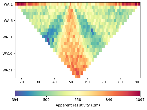
ert.show(syn_data)

Synthetic ERT Data Visualization

This plot shows a single timestep of synthetic ERT measurements. The data represents apparent resistivity values measured at different electrode configurations. Each point corresponds to a specific current injection and voltage measurement pair, providing information about subsurface resistivity distribution at this particular time.

%%

load all synthetic data and plot them

all_syn_data = []
for i in range(Water_Content.shape[0]):
    try:
        syn_data = pg.load(os.path.join(output_dir, "appres/synthetic_data" + str(i) + ".dat"))
        all_syn_data.append(np.array(syn_data['rhoa']))
    except Exception as e:
        print(f"Error loading synthetic data for timestep {i}: {e}")

## plot the apparent resitivity

import pandas as pd
import matplotlib.pylab as pylab
params = {'legend.fontsize': 13,
          #'figure.figsize': (15, 5),
         'axes.labelsize': 13,
         'axes.titlesize':13,
         'xtick.labelsize':13,
         'ytick.labelsize':13}

pylab.rcParams.update(params)
plt.rcParams["font.family"] = "Arial"


rng = pd.date_range(start="09/01/2011", end="08/30/2012", freq="D")
precip = np.load(os.path.join(data_dir, "precip.npy"))
syn_data_array = np.array(all_syn_data)
syn_data_array.shape



plt.figure(figsize=(12, 6))
plt.subplot(211)
plt.bar(np.arange(365),precip,color='k')
plt.xlim([0,364])
plt.ylabel('Precipitation (mm)')
plt.xlabel('Time (days)')
plt.subplot(212)
plt.imshow(syn_data_array.T, aspect='auto', cmap=pg.utils.cMap('rhoa'), vmin=200, vmax=2000)
plt.ylabel('Measurement #')
plt.xlabel('Time (days)')
plt.tight_layout()
plt.savefig(os.path.join(output_dir, "apparent_resistivity.tiff"), dpi=300)

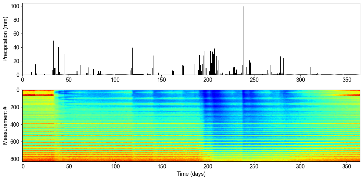
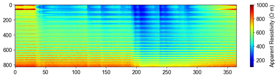
Time-Lapse Apparent Resistivity Response

The time-series analysis reveals the relationship between precipitation events and subsurface electrical response. The top panel shows daily precipitation over one year, while the bottom panel displays the corresponding apparent resistivity measurements for all electrode configurations. Notice how resistivity decreases (becomes more conductive) following major precipitation events, indicating increased water content in the subsurface.

%%

plt.figure(figsize=(12, 6))
plt.subplot(211)
plt.imshow(syn_data_array.T, aspect='auto', cmap=pg.utils.cMap('rhoa'), vmin=200, vmax=2000)
plt.colorbar(label='Apparent Resistivity (Ω·m)')

%%

## Showing the water content model for the differnent timesteps

fig, axes = plt.subplots(1, 4, figsize=(16, 14))

from palettable.lightbartlein.diverging import BlueDarkRed18_18_r
fixed_cmap = BlueDarkRed18_18_r.mpl_colormap
ax1 = axes[0]
wc25 = np.load(os.path.join(output_dir, "synwcmodel/synwcmodel30.npy"  ))
cbar1 = pg.show(mesh, wc25, ax=ax1, cMap=fixed_cmap, logScale=False,
              cMin=0.0, cMax=0.32, label='Water Content (-)',xlabel='Distance (m)', ylabel='Elevation (m)')
ax1.set_title("Day 30")


ax1 = axes[1]
wc150= np.load(os.path.join(output_dir, "synwcmodel/synwcmodel150.npy"  ))
cbar1 = pg.show(mesh, wc150, ax=ax1, cMap=fixed_cmap, logScale=False,
              cMin=0.0, cMax=0.32, label='Water Content (-)',xlabel='Distance (m)', ylabel='Elevation (m)')
ax1.set_title("Day 150")


ax1 = axes[2]
wc210= np.load(os.path.join(output_dir, "synwcmodel/synwcmodel210.npy"  ))
cbar1 = pg.show(mesh, wc210, ax=ax1, cMap=fixed_cmap, logScale=False,
              cMin=0.0, cMax=0.32, label='Water Content (-)',xlabel='Distance (m)', ylabel='Elevation (m)')
ax1.set_title("Day 210")


ax1 = axes[3]
wc280= np.load(os.path.join(output_dir, "synwcmodel/synwcmodel320.npy"  ))
cbar1 = pg.show(mesh, wc280, ax=ax1, cMap=fixed_cmap, logScale=False,
              cMin=0.0, cMax=0.32, label='Water Content (-)',xlabel='Distance (m)', ylabel='Elevation (m)')
ax1.set_title("Day 330")

fig.tight_layout()
plt.savefig(os.path.join(output_dir, "water_content_model.tiff"), dpi=300)

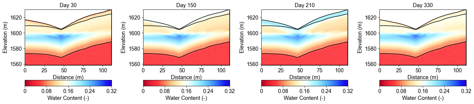
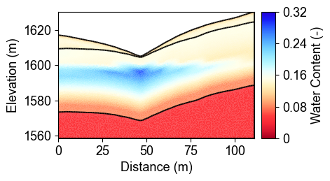
Water Content Evolution Over Time

These cross-sections show how water content changes throughout the year at four representative time points. Day 30 shows relatively dry conditions, Day 150 captures the wet season response, Day 210 represents peak saturation after sustained precipitation, and Day 330 shows the transition to drier conditions. Notice how water infiltrates from the surface (regolith layer) and gradually saturates deeper layers (fractured and fresh bedrock).

%% ## Showing the water content model for the differnent timesteps

fig, axes = plt.subplots(1, 4, figsize=(16, 14))

from palettable.lightbartlein.diverging import BlueDarkRed18_18
fixed_cmap = BlueDarkRed18_18.mpl_colormap
ax1 = axes[0]
wc30 = np.load(os.path.join(output_dir, "synresmodel/synresmodel30.npy"  ))
cbar1 = pg.show(mesh, wc30, ax=ax1, cMap=fixed_cmap, logScale=False, showColorBar=True,
        xlabel="Distance (m)", ylabel="Elevation (m)",
        label='Resistivity (Ω·m)', cMin=100, cMax=3000)



ax1 = axes[1]
wc150= np.load(os.path.join(output_dir, "synresmodel/synresmodel150.npy"  ))
cbar1 = pg.show(mesh, wc150, ax=ax1, cMap=fixed_cmap, logScale=False, showColorBar=True,
        xlabel="Distance (m)", ylabel="Elevation (m)",
        label='Resistivity (Ω·m)', cMin=100, cMax=3000)



ax1 = axes[2]
wc210= np.load(os.path.join(output_dir, "synresmodel/synresmodel210.npy"  ))
cbar1 = pg.show(mesh, wc210, ax=ax1, cMap=fixed_cmap,
              logScale=False, showColorBar=True,
        xlabel="Distance (m)", ylabel="Elevation (m)",
        label='Resistivity (Ω·m)', cMin=100, cMax=3000)


ax1 = axes[3]
wc280= np.load(os.path.join(output_dir, "synresmodel/synresmodel330.npy"  ))
cbar1 = pg.show(mesh, wc280, ax=ax1, cMap=fixed_cmap, logScale=False, showColorBar=True,
        xlabel="Distance (m)", ylabel="Elevation (m)",
        label='Resistivity (Ω·m)', cMin=100, cMax=3000)


fig.tight_layout()
plt.savefig(os.path.join(output_dir, "resistivity_model.tiff"), dpi=300)

Resistivity Model Evolution

The corresponding resistivity models show the inverse relationship with water content - high resistivity zones (red/yellow) indicate dry conditions while low resistivity areas (blue) represent saturated regions. The petrophysical transformation from water content to resistivity uses layer-specific parameters (formation resistivity, cementation exponent) that account for different geological units. This resistivity evolution serves as the basis for forward modeling synthetic ERT measurements.

%%

import numpy as np
import matplotlib.pyplot as plt
import os
from PIL import Image
import io

# Import your color map
from palettable.lightbartlein.diverging import BlueDarkRed18_18_r
fixed_cmap = BlueDarkRed18_18_r.mpl_colormap

# Create a list to store the frames
frames = []

# Set the DPI for consistent figure size
dpi = 100

# Create frames and store them in memory
for i in range(365):
    # Print progress update
    if i % 10 == 0:
        print(f"Processing frame {i} of 365")

    # Set up new figure for each frame - reduced height to eliminate empty space
    fig = plt.figure(figsize=[8, 2.2])

    # Use more of the figure space
    plt.subplots_adjust(left=0.05, right=0.95, top=0.95, bottom=0.05)

    ax = fig.add_subplot(1, 1, 1)

    # Load data
    moi = np.load(os.path.join(output_dir, f"synwcmodel/synwcmodel{i}.npy"))

    # Plot the data
    ax, cbar = pg.show(mesh, moi, pad=0.3, orientation="vertical",
                     cMap=fixed_cmap, cMin=0.00, cMax=0.32,
                     xlabel="", ylabel="",  # Remove labels to save space
                     label='Water content', ax=ax)

    # Style adjustments
    ax.spines['top'].set_visible(False)
    ax.spines['right'].set_visible(False)
    ax.spines['bottom'].set_visible(False)
    ax.spines['left'].set_visible(False)
    ax.get_xaxis().set_ticks([])
    ax.get_yaxis().set_ticks([])

    # Add day counter with better positioning and visibility
    # Use transAxes to position the text in a consistent location
    ax.text(0.1, 0.1, f'Day: {i}', transform=ax.transAxes,
            fontsize=12, fontweight='bold', color='black',
            bbox=dict(facecolor='white', alpha=0.7, edgecolor='none', pad=3))

    # Add compact axis labels
    ax.text(0.5, 0.02, 'Distance (m)', transform=ax.transAxes,
            ha='center', fontsize=8)
    ax.text(0.02, 0.5, 'Elevation (m)', transform=ax.transAxes,
            va='center', rotation=90, fontsize=8)

    # Save to buffer instead of file
    buf = io.BytesIO()
    plt.savefig(buf, format='png', dpi=dpi, bbox_inches='tight')
    plt.close(fig)  # Close the figure

    # Convert buffer to image and append to frames
    buf.seek(0)
    img = Image.open(buf)
    frames.append(img.copy())  # Copy the image to ensure it stays in memory
    buf.close()

print("All frames processed!")

# Save as GIF
gif_path = os.path.join(output_dir, "WCanimation.gif")
# The first frame's duration will be longer (500ms) to show initial state
durations = [500] + [100] * (len(frames) - 1)  # 100ms per frame after the first

# Save the GIF with optimized settings
frames[0].save(
    gif_path,
    format='GIF',
    append_images=frames[1:],
    save_all=True,
    duration=durations,
    loop=0,  # 0 means loop forever
    optimize=True
)

print(f"GIF saved successfully to {gif_path}")

Animation and Advanced Visualization

The code also generates an animated GIF showing the complete temporal evolution of water content throughout the year. This animation provides insights into:

• Seasonal patterns: Clear wet and dry season variations

• Infiltration dynamics: How water moves from surface to depth

• Layer interactions: Different response rates in geological units

• Event-based changes: Rapid responses to individual storms

The animation is saved as ‘WCanimation.gif’ in the results directory.

Summary and Applications

This example demonstrated the complete workflow for creating synthetic time-lapse ERT measurements from hydrological model outputs:

Key Workflow Steps:

1. Load and process MODFLOW water content time series

2. Interpolate 3D data to 2D profiles for geophysical modeling

3. Convert water content to resistivity using petrophysical models

4. Generate synthetic ERT data via forward modeling

5. Visualize temporal patterns in apparent resistivity

6. Create animations showing subsurface dynamics

Scientific Insights:

• ERT measurements show clear sensitivity to hydrological changes

• Temporal regularization is crucial for time-lapse inversions

• Multi-layer petrophysical models capture geological heterogeneity

• Parallel processing enables efficient large dataset generation

Next Steps:

• Apply time-lapse inversion techniques (see Ex_TL_inversion.py)

• Include structural constraints from seismic data

• Implement uncertainty quantification methods

• Integrate with real field measurements for validation

This synthetic dataset provides a controlled environment for testing and validating time-lapse ERT monitoring approaches in watershed applications.