Ex. Loading and Processing Hydrological Model Outputs

This example demonstrates how to load and process outputs from different hydrological models using PyHydroGeophysX. We show examples for both ParFlow and MODFLOW models.

The example covers: - Loading ParFlow saturation and porosity data - Loading MODFLOW water content and porosity data - Basic visualization of the loaded data

This is typically the first step in any workflow where you want to convert hydrological model outputs to geophysical data.

import os
import sys
import numpy as np
import matplotlib.pyplot as plt

# For Jupyter notebooks, use the current working directory
try:
    # For regular Python scripts
    current_dir = os.path.dirname(os.path.abspath(__file__))
except NameError:
    # For Jupyter notebooks
    current_dir = os.getcwd()

# Add the parent directory (OPEN_ERT) to the path
parent_dir = os.path.dirname(os.path.dirname(current_dir))
if parent_dir not in sys.path:
    sys.path.append(parent_dir)

from PyHydroGeophysX.model_output.parflow_output import ParflowSaturation, ParflowPorosity
from PyHydroGeophysX.model_output.modflow_output import MODFLOWWaterContent, MODFLOWPorosity

1. ParFlow Example

Let’s start by loading ParFlow data. ParFlow is a physically-based, three-dimensional model that simulates surface and subsurface flow.

Path to your Parflow model directory

current_dir = os.getcwd()
model_directory = os.path.join(current_dir, "data", "parflow", "test2")

# Load saturation data
saturation_processor = ParflowSaturation(
    model_directory=model_directory,
    run_name="test2"
)
saturation = saturation_processor.load_timestep(200)  # Load first timestep

# Load porosity data
porosity_processor = ParflowPorosity(
    model_directory=model_directory,
    run_name="test2"
)
porosity = porosity_processor.load_porosity()

mask = porosity_processor.load_mask()
mask.shape
porosity[mask==0] = np.nan
saturation[mask==0] = np.nan

print(saturation.shape)

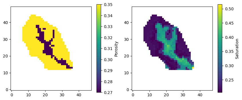
Visualizing ParFlow Data

Now let’s create visualizations of the loaded ParFlow data. We’ll plot both porosity and saturation for layer 19 of the model.

Plotting the data

plt.figure(figsize=(10, 4))
plt.subplot(1, 2, 1)
plt.imshow(porosity[19, :, :], cmap='viridis')
plt.colorbar(label='Porosity')
plt.gca().invert_yaxis()
plt.title('ParFlow Porosity (Layer 19)')

plt.subplot(1, 2, 2)
plt.imshow(saturation[19, :, :], cmap='viridis')
plt.colorbar(label='Saturation')
plt.gca().invert_yaxis()
plt.title('ParFlow Saturation (Layer 19)')

plt.tight_layout()
plt.show()

The above plot shows the porosity and saturation data from ParFlow simulation. Notice how the values vary spatially across the domain. The porosity shows the void space available for fluid storage, while saturation indicates how much of that space is filled with water.

2. MODFLOW Example

MODFLOW is a widely-used groundwater flow model. Here we’ll load water content and porosity data from a MODFLOW simulation.

These would be your actual data files

data_dir = model_directory = os.path.join(current_dir, "data")
modflow_dir = os.path.join(data_dir, "modflow")
idomain = np.loadtxt(os.path.join(modflow_dir, "id.txt"))

# Initialize MODFLOW water content processor
water_content_processor = MODFLOWWaterContent(
    model_directory=modflow_dir,  # Changed from sim_ws
    idomain=idomain
)

# Load water content for a specific timestep
timestep = 1
water_content = water_content_processor.load_timestep(timestep)

print(water_content.shape)

# Path to your MODFLOW model directory
model_name = "TLnewtest2sfb2"  # Your model name

# 1. Create an instance of the MODFLOWPorosity class
porosity_loader = MODFLOWPorosity(
    model_directory=modflow_dir,
    model_name=model_name
)
# 2. Load the porosity data
porosity_data = porosity_loader.load_porosity()

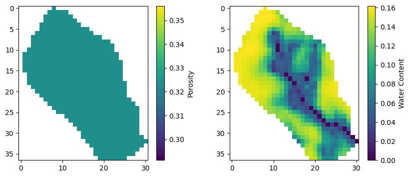
Visualizing MODFLOW Data

Let’s create visualizations of the MODFLOW simulation results. We’ll compare the porosity distribution with the water content.

Plotting the data

porosity_data1 = porosity_data[0, :, :]
porosity_data1[idomain==0] = np.nan

plt.figure(figsize=(10, 4))
plt.subplot(1, 2, 1)
plt.imshow(porosity_data1[ :, :], cmap='viridis')
plt.colorbar(label='Porosity')
plt.title('MODFLOW Porosity')

plt.subplot(1, 2, 2)
plt.imshow(water_content[0, :, :], cmap='viridis')
plt.colorbar(label='Water Content')
plt.title('MODFLOW Water Content')

plt.tight_layout()
plt.show()

The MODFLOW results show the comparison between porosity distribution and water content. The water content represents the volumetric water content, which is the product of porosity and saturation.

Summary and Next Steps

This example has demonstrated the basic workflow for loading hydrological model outputs using PyHydroGeophysX. Key points:

ParFlow Integration: Load 3D saturation and porosity fields from ParFlow simulations
MODFLOW Integration: Access water content and porosity from MODFLOW models
Data Visualization: Create plots to understand spatial distribution of properties
Data Preprocessing: Handle inactive cells and missing data appropriately

The loaded hydrological data serves as input for geophysical forward modeling, where water content and porosity are converted to resistivity and seismic velocity using petrophysical relationships.