
Desktop Workbench (Qt)#
PyHydroGeophysX ships two complementary front ends:
The Streamlit web app (Agent Web App) is the agent, report, tutorial, and deployment portal. It runs in a browser and can be hosted remotely.
The Qt desktop workbench (
PyHydroGeophysX/qt_apps/) is a local desktop application for hands-on mouse interaction: data processing, first-arrival picking, electrode geometry editing, hydro-to-geophysics profile selection, mesh building, and forward modeling and inversion.
The two exchange small JSON files on disk (the “bridge”), so you can set up a run in the browser and finish the interactive work on the desktop.
Workbench at a Glance#
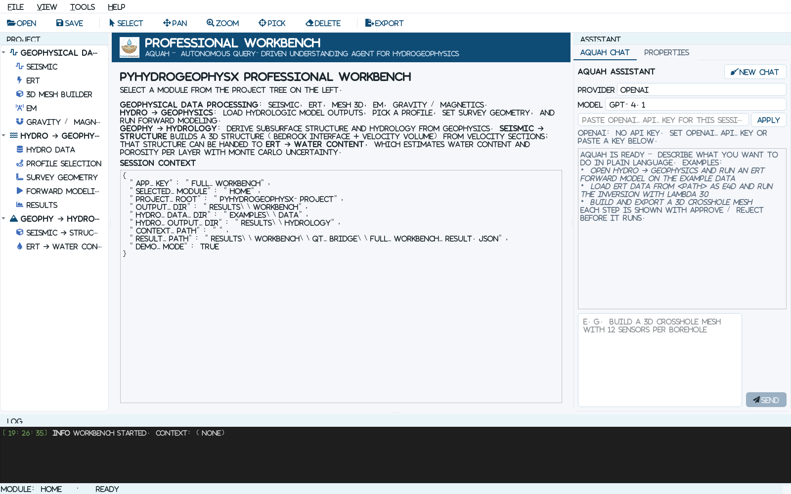
The Workbench home screen. The project tree is on the left, the active scientific module is in the center, AQUAH Chat and Properties are on the right, and the activity log is at the bottom.#
The main window has six working areas:
Project tree – select Seismic, ERT, 3D Mesh Builder, EM, Gravity / Magnetics, Hydro -> Geophysics, Seismic -> Structure, or ERT -> Water Content. Multiple tree entries under Hydro -> Geophysics open different stages of the same guided module.
Module workspace – plots, maps, model viewers, and step-by-step controls for the selected method.
AQUAH Chat / Properties – ask the assistant to prepare an action, or inspect the current context and module results as JSON.
Toolbar – Open, Save, Select, Pan, Zoom, Pick, Delete, and Export. Pick and Delete act on compatible plots in the active module.
Log – progress messages, loaded-file summaries, warnings, output paths, and backend errors. Check this panel first when a run does not start.
Status bar – the current module and whether the interface is ready or busy.
Download the Desktop App#
Prebuilt bundles for Windows and macOS are published on GitHub Releases. Each platform has two variants, so you can pick what fits your machine:
Download the Desktop Workbench (Windows / macOS)
Bundle |
What it includes |
|---|---|
|
Windows. Load, view, QC, pick, edit geometry, and export data in every module. Small download; starts fast. |
|
Windows. Everything in light, plus the geophysics engines (PyGIMLi, SimPEG, PyVista/VTK): forward modeling, inversion, and the 3D mesh viewer work out of the box. Much larger download. |
|
macOS. Same feature set as the Windows light build. |
|
macOS. Same feature set as the Windows full build. |
After unzipping, run PyHydroGeophysX-Workbench.exe inside the extracted folder
(Windows) or open PyHydroGeophysX-Workbench.app (macOS).
Note
In the light bundles the heavy engines are left out on purpose, so forward modeling, inversion, and the 3D mesh viewer show an install message instead of running. Choose the full bundle, or install from source, for the complete feature set.
Note
The macOS bundles are not code-signed. If macOS blocks the first launch,
right-click the app and choose Open once, or clear the quarantine flag with
xattr -cr PyHydroGeophysX-Workbench.app.
Install and Run from Source#
The workbench needs PySide6 and pyqtgraph in addition to numpy and pandas:
pip install -r requirements-desktop.txt
# or, as an extra:
pip install "pyhydrogeophysx[desktop]"
Optional packages add features:
pygimli: real forward modeling and inversion (ERT, SRT, TDEM, FDEM, gravity). Without it, the Hydro module still exports a survey configuration JSON.pyvista,pyvistaqt,vtk: the 3D mesh viewer.simpeg: gravity and magnetics 3D inversion.scipy: gridding and interpolation in several modules.
Launch the workbench:
python -m PyHydroGeophysX.qt_apps.launcher

# open directly into a module:
python -m PyHydroGeophysX.qt_apps.launcher --module hydro_geophysics

# attach to a bridge context written by Streamlit:
python -m PyHydroGeophysX.qt_apps.launcher --context results/streamlit_workflow/qt_bridge/full_workbench_context.json
If the package is installed (pip install pyhydrogeophysx[desktop]), the
pyhydrogeophysx-workbench command starts the same application. Helper scripts are
provided in scripts/: start_qt_workbench.bat (Windows) and
start_qt_workbench.sh (macOS / Linux).
Module keys for --module: home, seismic, ert, mesh3d, em,
gravmag, hydro_geophysics, geo_hydrology, seismic3d.
Your First Workbench Run: ERT Inversion#
This walkthrough uses the ERT module because it demonstrates the complete
Workbench pattern: load, inspect, QC, configure, run, evaluate, and export. From
a source checkout, use examples/data/ERT/Bert/fielddataline2.dat. You can use
your own BERT/unified, E4D, Syscal, or other supported resistivity file instead.
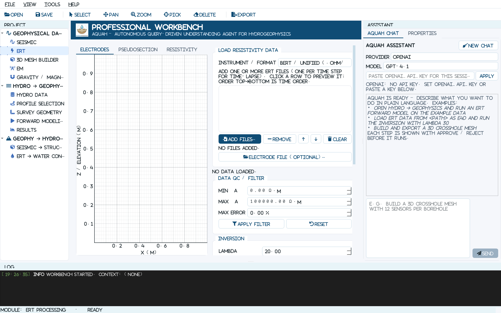
The ERT Processing module before a file is loaded. Data and result tabs are on the left; loading, filtering, inversion, editing, and export controls are in the scrollable center panel.#
Step 1 – open the ERT module#
Select Geophysical Data Processing > ERT in the project tree, or launch directly with:
python -m PyHydroGeophysX.qt_apps.launcher --module ert
Step 2 – load and inspect data#
Under Load resistivity data, select the matching Instrument / format. For the bundled file, choose BERT / Unified (.ohm/.dat).
Click Add files… and select one file. Loading runs in a worker thread; the UI remains responsive and the Log reports the number of electrodes and measurements.
Use the Electrodes tab to check positions and elevation. Use Pseudosection to inspect spatial coverage and apparent-resistivity outliers.
If electrode positions are stored separately, click Electrode file (optional)…. The Workbench accepts an
x, ztable.
Step 3 – apply QC filters#
Set Min rhoa, Max rhoa, and optionally Max error, then click Apply filter. A Max error value of zero disables the error filter. The Log reports how many measurements were retained and removed. Click Reset to return to the original loaded data before trying different thresholds.
Do not use a narrow resistivity range simply to make a smooth-looking plot. Check suspicious points against acquisition notes, reciprocal error, contact resistance, and neighboring measurements before deleting them.
Step 4 – configure and run the inversion#
The defaults provide a reasonable first diagnostic run:
Lambda = 20 controls spatial smoothness. Increase it for a smoother model; decrease it only when the data quality and coverage justify more structure.
Max iterations = 15 limits the Gauss-Newton iterations.
Relative error = 0.05 assigns a 5% data error for weighting.
Mesh quality = 34 controls the inversion triangulation.
Click Run inversion. Follow progress in the bottom Log. When the run finishes, inspect:
Resistivity model for the recovered section and coverage-aware opacity;
Inversion quality for observed-versus-predicted behavior and convergence;
the Log for the final chi-squared value and saved intermediate paths.
Step 5 – edit geometry and export#
Use Add electrode (click to place) or Edit (click select, click move) only when the geometry needs correction. Right-click an electrode to delete it or change its label. Then export one or more of:
Export electrode file… for the corrected coordinate table;
Export survey geometry JSON… for a reusable survey definition;
Export resistivity model… for
.npy, PyGIMLi.bms, and VTK files.
Use File > Save Workbench Result to save the cross-module result JSON used by the Streamlit bridge. This is different from exporting the scientific model files above.
Time-Lapse ERT#
The ERT loader also manages an ordered time series:
Click Add files… and select two or more ERT files. Each file represents one time step.
Verify that the list is chronological. Use the up and down arrow buttons to reorder selected rows. Clicking a row previews that time step.
Check Time-lapse (multiple ERT files). The temporal controls appear.
Set Alpha (temporal), then choose L2 for smooth changes, L1 for blockier changes, or L1L2 for the hybrid formulation.
For long sequences, enable Windowed (sliding window) and choose a window size, or enable Low memory (sparse). Low-memory mode is also selected automatically for sufficiently large problems.
Click Run time-lapse inversion. After completion, select time steps in the Resistivity model tab and click Export results (VTK + npy + mesh)… to save combined and per-step VTK files,
final_models.npy, the mesh, acquisition times, and the result figure.
Module-by-Module Workflows#
Each module follows the same left-to-right logic. The shortest reliable path through each one is summarized below.
Module |
Recommended sequence |
Main outputs |
|---|---|---|
Seismic Processing |
Load a gather; load positions/topography if available; set shot and receiver geometry; adjust gain, clipping, polarity, normalization, and AGC; auto-pick or manually pick first arrivals; inspect the Travel-time tab; run SRT inversion. |
Picks CSV, PyGIMLi travel-time |
3D Mesh Builder |
Choose surface-grid, borehole, or crosshole geometry; select mesh engine and topography; set domain and refinement; click 1. Preview sensors; then 2. Generate mesh; inspect the 3D viewer. |
BMS, VTK, sensor CSV, and a reusable survey/mesh configuration. |
EM Processing |
Select FDEM or TDEM; load one or multiple soundings; load line geometry when available; confirm system geometry; configure the 1D Occam inversion; click Run inversion; compare Sounding, Resistivity model, and Inversion quality tabs. |
Recovered model |
Gravity / Magnetics |
Load |
Corrected/QC data, density or susceptibility model, NPZ/VTK, and convergence history. |
Hydro -> Geophysics |
Data: use example/context data or select the hydrologic-output folder. Profile: pick two map points. Methods: select ERT, SRT, EM, or gravity. Parameters: review petrophysics and survey settings. Run: confirm the readiness checklist and run forward modeling. |
Extracted profile, survey configurations, synthetic responses, models, and figures for each selected method. |
Seismic -> Structure |
Load velocity sections and line coordinates; set interface threshold; preview the first interface; configure interpolation/grid options; check Readiness; click Build 3D model. |
Bedrock surface, 3D velocity/structure volume, configuration JSON, and a direct handoff to ERT -> Water Content. |
ERT -> Water Content |
Load a model folder containing |
Mean, standard deviation, percentile models, layer summaries, monitoring-point time series, and petrophysics configuration JSON. |
Using AQUAH Chat Safely#
The right-side AQUAH Chat tab can navigate modules, load example data, change parameters, and start supported actions.
Select OpenAI, Anthropic, or an OpenAI-compatible provider and model.
Paste an API key for the current session or set the provider’s environment variable before launch.
Describe one concrete task, for example:
Open ERT, load the bundled BERT line, set lambda to 20, and prepare an inversion.Review every proposed tool action. Click Approve only when the file, parameters, output directory, and operation are correct; otherwise click Reject and revise the request.
Confirm completion in the module itself and in the Log. Chat does not replace inspection of the data or inversion-quality plots.
Saving, Exporting, and Reopening Work#
File > Save Workbench Result writes
full_workbench_result.jsonfor the web/desktop bridge.File > Export Current Module Result… writes the current module’s JSON-serializable summary.
Module-specific Export buttons save scientific arrays, meshes, VTK files, tables, and figures.
File > Open Project Context… reopens a bridge context JSON and rebuilds module pages against that project.
Window geometry and dock positions persist between sessions. Use View > Reset Layout if a dock is hidden or misplaced.
Modules#
Module |
What it does |
|---|---|
Seismic Processing |
Load 2D shot gathers (SEG-Y, Geometrics DAT), apply gain / AGC / normalization, pick first arrivals (assisted auto-picking plus manual and line picking), QC travel times, and run SRT travel-time tomography. Pre-picked travel-time files can be uploaded and inverted directly. |
ERT Processing |
Load resistivity files by instrument format (BERT / unified, E4D, Syscal, and more), edit electrodes, QC the apparent-resistivity pseudosection, filter data, and run single or time-lapse inversion with per-step results. |
3D Mesh Builder |
Build ERT meshes (surface grid, borehole, crosshole arrays; flat, tilted, Gaussian-hill, file-based, or custom topography), view meshes in 3D with a clipping plane, and run 3D ERT forward modeling on the generated mesh. |
EM Processing |
Load TDEM / FDEM soundings (single or multi-sounding line files), invert one sounding or a whole line into a stitched resistivity section, and view plan-view depth-slice maps on survey coordinates. |
Gravity / Magnetics |
Load station data, remove regional trends, and run SimPEG 3D inversion with an interactive model viewer. |
Hydro -> Geophysics |
Load hydrologic model outputs (water content, porosity, surfaces), pick a profile, set petrophysical parameters, and run forward modeling for the selected geophysical methods. |
ERT -> Water Content |
Invert ERT results into water content estimates. |
Seismic -> Structure |
Derive 3D structural surfaces from seismic lines. |
The workbench also includes AQUAH Chat, an in-app assistant that can drive the modules through natural language (OpenAI, Anthropic, or any OpenAI-compatible provider; bring your own API key). Every proposed action shows an Approve / Reject button before it runs.
How the Streamlit / Qt Bridge Works#
The bridge directory is <output_dir>/qt_bridge/ (default
results/streamlit_workflow/qt_bridge/).
In the web app’s Professional Workbench tab, a launch button writes
full_workbench_context.json(project root, output directory, hydro data directory, current workflow configuration and result, and the Python executable to reuse).Streamlit starts the Qt workbench as a separate process and passes that context path.
The Qt app reads the context on startup, so it points at the same project and data.
When you save in the Qt app (File -> Save Workbench Result, or after a forward run), it writes
full_workbench_result.jsonwith the per-module results.Back in the browser, the results panel reads that file and displays it.
Modules can also export their own files (picks CSV, electrode geometry JSON, processed EM curves, corrected gravity data, survey configuration JSON, figures) into the output directory.
Remote Servers and Download Mode#
A Qt window opens on the machine where the Python process runs. When Streamlit is hosted on a remote server, that server has no display attached to your screen, so the Professional Workbench tab switches to download mode and shows the download links above instead of launch buttons. The default links point at the latest GitHub Release and can be overridden with environment variables:
PHGX_QT_DOWNLOAD_WINDOWSPHGX_QT_DOWNLOAD_MACOSPHGX_QT_DOWNLOAD_LINUXPHGX_QT_DOWNLOAD_SOURCE
PHGX_FORCE_REMOTE_MODE=1 forces download mode; PHGX_ENABLE_LOCAL_QT=1 opts in
to a local launch when PySide6 is present.
Persistence and Troubleshooting#
Window size and dock layout persist between sessions via
QSettings(organization “PyHydroGeophysX”, application “Workbench”). Delete that settings key to reset the layout to defaults.Uncaught errors show a dialog with a copyable traceback instead of closing the app silently; the same text also goes to stderr and can be reported as a GitHub issue.
If a module page shows a “could not be loaded” message, it names the missing optional package and the install command; the rest of the workbench is unaffected.
Building the Bundles Yourself#
The PyInstaller configuration lives at packaging/pyinstaller_workbench.spec. The
PHGX_BUILD_VARIANT environment variable selects light (default) or full.
Helper scripts build and zip a bundle in one step:
# Windows (PowerShell)
scripts/build_workbench_exe.ps1 light

# macOS / Linux
bash scripts/build_workbench_exe.sh light
The GitHub Actions workflow .github/workflows/build-desktop.yml builds all four
bundles and attaches them to the Release for every version tag.